Zernikes

Prysm supports several flavors of Zernike polynomial: - Fringe - Noll - ANSI “j” - ANSI “n,m”

The single index notations have identical interfaces, while the (n,m) notation is slightly different.

Zernike notations are a subclass of Pupil, so they support the same arguments to __init__,

%matplotlib inline
from prysm import FringeZernike, NollZernike, ANSI1TermZernike, ANSI2TermZernike
p = FringeZernike(samples=123, dia=456.7, wavelength=1.0, z_unit='nm', phase_mask='dodecagon')

There are additional keyword arguments for each term. The polynomials are orthogonal, having unit amplitude (zero-to-peak). They can also be used with unit variance via the norm keyword argument, in which case they are orthonormal. The polynomial classes have friendly print statements:

p2 = FringeZernike(Z4=1, Z9=1, Z98=1, norm=True)
print(p2)

rms normalized Fringe Zernike description with:
        +1.000 Z4 - Defocus
        +1.000 Z9 - Primary Spherical
        +1.000 Z98 - 8th Coma Y
        11.758 PV, 1.718 RMS [nm]

Notice that we include a 98th term which you likely will not find in most other programs, and that the RMS value is equal to sqrt(1^2 + 1^2 + 1^2) = sqrt(3) = 1.718 ~= 1.722. The difference is due to the array sizes used by prysm by default, if increased, e.g. by adding samples=1204 to the constructor, the value would converge to the analytical one.

A Zernike pupil can also be initalized with an iterable (list, tuple…) of coefficients,

import numpy as np
terms = np.random.rand(49)  # 49 zernike coefficients, e.g. from a wavefront sensor
fz3 = FringeZernike(terms)

Zernike instances have a truncate method which discards terms with indices higher than n. For example,

fz3.truncate(16)
print(fz3)

Fringe Zernike description with:
        +0.237 Z1 - Piston
        +0.422 Z2 - Tilt Y
        +0.150 Z3 - Tilt X
        +0.859 Z4 - Defocus
        +0.073 Z5 - Primary Astigmatism 00°
        +0.757 Z6 - Primary Astigmatism 45°
        +0.475 Z7 - Primary Coma Y
        +0.522 Z8 - Primary Coma X
        +0.579 Z9 - Primary Spherical
        +0.198 Z10 - Primary Trefoil Y
        +0.832 Z11 - Primary Trefoil X
        +0.588 Z12 - Secondary Astigmatism 00°
        +0.527 Z13 - Secondary Astigmatism 45°
        +0.916 Z14 - Secondary Coma Y
        +0.381 Z15 - Secondary Coma X
        +0.202 Z16 - Secondary Spherical
        +0.825 Z17 - Primary Quadrafoil 00°
        60.920 PV, 4.473 RMS [nm]

fz3.top_n(5)

[(0.91562805153131, 14, 'Secondary Coma Y'),
 (0.8587566090731925, 4, 'Defocus'),
 (0.8315043074143359, 11, 'Primary Trefoil X'),
 (0.8247641831374353, 17, 'Primary Quadrafoil 00°'),
 (0.7565978303965777, 6, 'Primary Astigmatism 45°')]

or the terms listed by their pairwise magnitudes and clocking angles,

fz3.magnitudes

{'Piston': (0.23745919086319245, 0),
 'Tilt': (0.44849286815677, 70.39346804745544),
 'Defocus': (0.8587566090731925, 0),
 'Primary Astigmatism': (0.7600997704834245, 5.502037764188377),
 'Primary Coma': (0.7061017606036157, 42.27652344562817),
 'Primary Spherical': (0.5791772079761679, 0),
 'Primary Trefoil': (0.8546972533464932, 13.378161550297573),
 'Secondary Astigmatism': (0.7898356917600361, 48.13921037292902),
 'Secondary Coma': (0.9916106766946162, 67.42451186641055),
 'Secondary Spherical': (0.20220097264202486, 0),
 'Primary Quadrafoil': (0.8247641831374353, 0)}

Magnitudes is a dict keyed by the name with values of (mag, ang). The angle is always zero if the term is rotationally invariant.

These things may be (bar) plotted;

fz3.barplot(orientation='h', buffer=1, zorder=3)
fz3.barplot_magnitudes(orientation='h', buffer=1, zorder=3)
fz3.barplot_topn(n=5, orientation='h', buffer=1, zorder=3)

(<Figure size 432x288 with 1 Axes>,
 <matplotlib.axes._subplots.AxesSubplot at 0x7f7750984eb8>)

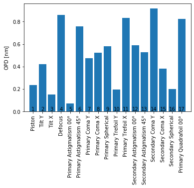
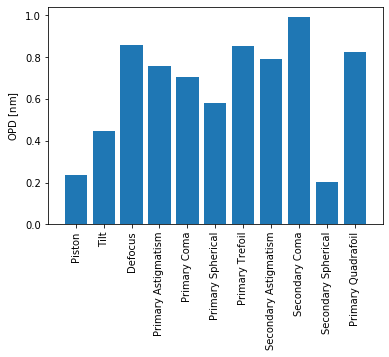
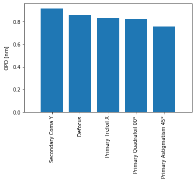
orientation controls the axis on which the terms are enumerated. h results in vertical bars, v is also accepted, as are horizontal and vertical. buffer is the number of terms’ worth of spaces left on each side. The default of 1 leaves a one bar margin. zorder is passed to matplotlib – the default of 3 places the bars above any gridlines, which is an aesthetic choice. Matplotlib has a general default of 1.

If you would like direct access to the underlying functions, the first few polynomials are provided as explicit functions and can be imported:

from prysm.zernike import defocus

each of these takes arguments of (rho, phi). They have names which end with _x, or _00 and _45 for the terms which have that naming convention.

Zernike functions are cached by prysm’s internal routines,

from prysm.zernike import zcachemn
# 8 is the index into prysm.zernike.zernikes, which loosely follows the Fringe ordering
zcachemn(7, 7, norm=True, samples=128)
zcachemn.clear()  # you should never have to do this unless you want to release memory

This cache instance is used internally by prysm, if you modify the returned arrays in-place, you probably won’t like the result. You can create your own independent instance,

from prysm.zernike import ZCacheMN
my_zcache = ZCacheMN()

See Pupils for information about general pupil functions.