Single-Mode Fibers

This tutorial will demonstrate how to model optical fiber using prysm. We will begin by reverse engineering a commercial fiber in order to model its mode field then show an example of of a multi-mode fiber derived from first principles. We’ll begin with the single mode fiber, a ThorLabs SM400. The Manufacture provides the following specifications:

Specification	Value	Unit
Operating Wavelength	405 - 532	nm
Mode Field Diameter	2.5 - 3.4	um
Core Index at 467 nm	1.46435
Cladding Index at 467 nm	1.45857
Numerical Aperture	0.12 - 0.14
Cladding Diameter	125	um
Core Diameter	?	um

The reader is assumed to be familiar with the meaning of these parameters. The manufacture does not provide the core diameter, which is the first piece of needed information. The first useful functions from x/fibers will allow us to use the provided mode field diameter to bound the V-number of the fiber, which is a normalized frequency that determines how many modes can propagate in the fiber. A fiber with V < ~2.4048 is single mode.

import numpy as np

from matplotlib import pyplot as plt

from prysm.x.fibers import (
    numerical_aperture,
    V,
    marcuse_mfr_from_V,
    petermann_mfr_from_V
)

First we’ll check that the provided indices really do mean an NA between 0.12 and 0.14:

ncore = 1.46435
nclad = 1.45857
wvl = 0.467
na = numerical_aperture(ncore, nclad)
na

np.float64(0.12997875826457253)

The NA ishe NA is 0.13, square in the middle of the provided range. Because the indices vary with wavelength, so too does the NA. It is not surprising that for a wavelength in the middle of the specified operating range, the NA lands in the middle of the specified range. The function V is of the form def V(radius, NA, wavelength) and the first argument is not known. We can work backwards by finding a plausible V-number based on their parameters:

v_scan = np.linspace(1, 3, 100)
mfr_estimate = petermann_mfr_from_V(v_scan)
worse_mfr_estimate = marcuse_mfr_from_V(v_scan)

fig, ax = plt.subplots()
ax.plot(v_scan, mfr_estimate, zorder=2)
ax.plot(v_scan, worse_mfr_estimate, zorder=2)
ax.axvline(2.4048, ls='--', c='k', zorder=0)
ax.text(2.39, 3, 'Single Mode Cutoff', ha='right', va='center', rotation=90)
ax.set(xlabel='V-number', ylabel='(mode field radius)/(core radius)')
ax.legend(['Petermann', 'Marcuse'], title='Estimate')

<matplotlib.legend.Legend at 0x768734c5d010>

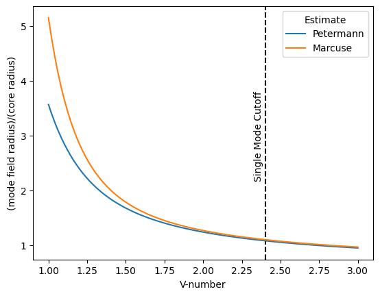
In order for the fiber to be single mode over the full range of specified wavelengths and have that property as manufactured with nonzero tolerances, the V-number needs to be somewhat less than the single mode cutoff. We’ll start with a guess of 2.1 and find the parameters for the (single) mode:

from prysm.x.fibers import find_all_modes

vv = 2.1
relative_mfr = petermann_mfr_from_V(vv)
spec_mfr = (2.5+3.4)/2/2 # average, assume falls in the middle
estimated_core_radius = spec_mfr/relative_mfr
modes = find_all_modes(V=vv)
print(f'{estimated_core_radius=:.1f}, {modes=}')

estimated_core_radius=1.2, modes={0: array([0.44758096])}

The return value of find_all_modes is a dictionary with keys of azimuthal order and values of lists of b-values or propagation constants (values between 0 and 1) for each mode. The fiber’s core must be about 5 microns in diameter. With these parameters we can calculate the mode of the fiber:

from prysm import coordinates
from prysm.x.fibers import smf_mode_field

x, y = coordinates.make_xy_grid(256, diameter=5*estimated_core_radius)
r, t = coordinates.cart_to_polar(x, y)

# modes[0][0] = the 0th order azimuthal mode, first mode (the only mode for a single mode fiber)
mode_field_2d = smf_mode_field(vv, estimated_core_radius, modes[0][0], r)

fig, ax = plt.subplots()
ax.imshow(mode_field_2d, extent=[x.min(), x.max(), y.min(), y.max()], cmap='inferno')
circ = plt.Circle((0,0), radius=estimated_core_radius, fill=False, lw=0.5, color='w', ls='--')
ax.add_artist(circ)
ax.text(-2.8, 2.5, 'Fiber Core', c='w')
ax.set(xlabel='X, um', ylabel='Y, um')

[Text(0.5, 0, 'X, um'), Text(0, 0.5, 'Y, um')]

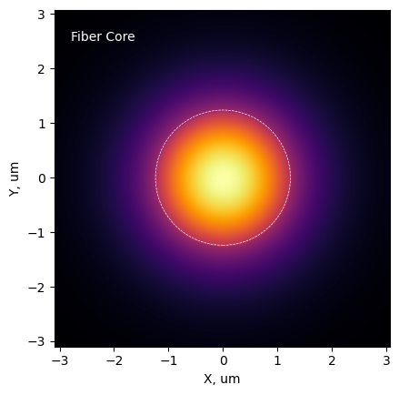
Note that the image is the complex electric field (which is purely real for an idealized single mode fiber), the intensity is the square of this and is what is usually observable. We can see that the mode is “weakly confined”, with significant energy in the cladding. This is entirely determined by Petermann’s equation. By using values provided at other wavelengths, we can further refine our estimate of the core radius.

# wvl, ncore, nclad
mfg_values = [
    (.405, 1.46958, 1.46382),
    (.467, 1.46435, 1.45857),
    (.532, 1.46071, 1.45491),
]
nas = []
v_numbers = []
print('wvl_nm NA      V-number')
for (wvl, ncore, nclad) in mfg_values:
    wvl_nm = int(wvl*1e3)
    na = numerical_aperture(ncore, nclad)
    vnum = V(estimated_core_radius, na, wvl)
    na_str = str(round(na, 5))
    v_str = str(round(vnum, 3))
    # <n is f-string fixed width formatting
    print(f'{wvl_nm:<6} {na_str:<7} {v_str:<5}')

wvl_nm NA      V-number
405    0.12999 2.498
467    0.12998 2.166
532    0.13004 1.902

We can see that with our estimated core radius, the fiber is single mode in the mid and long end of its specified band, not not near the lower end. We can run the calculation again with a reduced mode core radius which will produce just-barely single mode behavior at the short end of the specified bandpass:

revised_core_radius_guess = 1.15
print('wvl_nm NA      V-number')
for (wvl, ncore, nclad) in mfg_values:
    wvl_nm = int(wvl*1e3)
    na = numerical_aperture(ncore, nclad)
    vnum = V(revised_core_radius_guess, na, wvl)
    na_str = str(round(na, 5))
    v_str = str(round(vnum, 3))
    # <n is f-string fixed width formatting
    print(f'{wvl_nm:<6} {na_str:<7} {v_str:<5}')

wvl_nm NA      V-number
405    0.12999 2.319
467    0.12998 2.011
532    0.13004 1.766

We can create a psuedocolor image of the mode field in RGB:

rgb_modes = np.empty((*r.shape, 3), dtype=float)

j = 0
for (wvl, ncore, nclad) in mfg_values:
    na = numerical_aperture(ncore, nclad)
    vnum = V(revised_core_radius_guess, na, wvl)
    modes = find_all_modes(vnum)
    # normalize modes by the core area
    mode_field_2d = smf_mode_field(vnum, revised_core_radius_guess, modes[0][0], r)
    rgb_modes[:,:,j] = mode_field_2d
    j += 1

fig, ax = plt.subplots()
ax.imshow(rgb_modes/rgb_modes.max(), extent=[x.min(), x.max(), y.min(), y.max()])
ax.set(xlabel='X, um', ylabel='Y, um')

[Text(0.5, 0, 'X, um'), Text(0, 0.5, 'Y, um')]

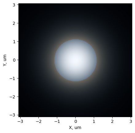
One can see that over the specified bandwidth, the fiber is largely but not entirely achromatic. The more red wavelengths have more energy outside of the core. We can conclude this exercvise by calculating the coupling efficiency of a perfect circular lens into the fiber as a function of wavelength:

from prysm.psf import airydisk_efield
from prysm.x.fibers import mode_overlap_integral

wvls = [.405, .467, .532]
# core radius ~ 1.2, need fno x lambda ~ 1.2; fno ~2 for decent coupling
fno = 2.

overlaps = []
for j, wvl in enumerate(wvls):
    fiber_mode = rgb_modes[...,j]
    airydisk = airydisk_efield(r, fno, wvl)
    airydisk /= airydisk.sum()
    eta = mode_overlap_integral(fiber_mode, airydisk)
    overlaps.append(eta)

/home/docs/checkouts/readthedocs.org/user_builds/prysm/conda/latest/lib/python3.14/site-packages/prysm/mathops.py:259: RuntimeWarning: invalid value encountered in divide
  out = _besselj1(r) / r

fig, ax = plt.subplots()

total_fiber_energy = rgb_modes.sum(axis=(0,1))

ax.plot(wvls, overlaps)
ax.plot(wvls, total_fiber_energy/40_000)
ax.legend(['Coupling Efficiency', 'Scaled area under fiber mode'])

<matplotlib.legend.Legend at 0x76872b131fd0>

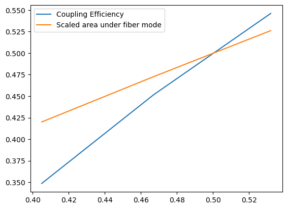
From the larger slope of the coupling efficiency curve, the fiber is somewhat achromatic but the chromaticity of diffraction means that coupling efficiency for a perfect lens is even more chromatic than the fiber. However, from the efficiency of ~45%, this is a significantly suboptimal F-number. We can repeat the calculation near a set of more optimal ones:

wvls = [.405, .467, .532]
# core radius ~ 1.2, need fno x lambda ~ 1.2; fno ~2 for decent coupling
fnos = [3.5, 4, 4.5]

overlaps = []
for j, wvl in enumerate(wvls):
    fiber_mode = rgb_modes[...,j]
    tmp = []
    for fno in fnos:
        airydisk = airydisk_efield(r, fno, wvl)
        airydisk /= airydisk.sum()
        eta = mode_overlap_integral(fiber_mode, airydisk)
        tmp.append(eta)

    overlaps.append(tmp)

fig, ax = plt.subplots()

ax.plot(wvls, overlaps)
# ax.plot(wvls, total_fiber_energy/40_000)
ax.legend(fnos, title='F#')
ax.set(xlabel='Wavelength, um', ylabel='Coupling efficiency eta')

[Text(0.5, 0, 'Wavelength, um'), Text(0, 0.5, 'Coupling efficiency eta')]

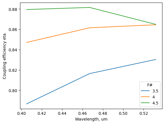
For near optimal coupling efficiencies the system is considerably more achromatic. And that the F-number is large enough that the airy disk’s first ring is significantly outside the core. This is again because the fiber mode has significant power outside the core.

Wrap-Up

In this tutorial, we looked at modeling single mode fibers. We started by reverse engineering missing parametric information from a vendor about their fiber, arriving at a plausible estimate for the core diameter. We then computed the mode field over a range of wavelengths as well as the coupling efficiency of a perfect circular lens into the fiber.