Optimization Basics

This tutorial will introduce the basics of optimization using prysm’s x/optym experimental module. We will:

1. Discuss the kind of optimization prysm is able to perform

2. Show how the machinery works using a common toy function

3. Use governors to stop optimization based on convergence instead of a fixed iteration count

At the end of this tutorial, you will be able to use x/optym to solve optimization problems.

Gradient-Based Optimization

All of the optimizers within prysm are gradient-based, meaning they require you be able to compute some scalar loss function \(\mathcal{L}(x)\), and its gradient \(\nabla = \langle \partial\mathcal{L}/\partial x_1,\partial\mathcal{L}/\partial x_2, \ldots, \partial\mathcal{L}/\partial x_N \rangle\). You may also see the loss function called an objective function, a merit function, or a cost function. You may also see the parameter vector \(x\) as a \(\theta\). prysm features only gradient-based optimizers, for gradient-free optimizers like Nelder-Meade or Hessian-based optimizers like Newton’s method, you will have to look elsewhere for now.

Computing \(\nabla\) may seem intractible on its face, but using algorithmic differentiation built into prysm, it is straightforward and most of the things you might want to differentiate with respect to are available batteries included today. We’ll start with a toy problem, the rosenbrock function from scipy.optimize, which is very difficult to minimize. Scipy includes both it and and its derivative, so we’ll import those:

from scipy.optimize import rosen, rosen_der

rosen is the \(\mathcal{L}(x)\) function itself, and rosen_der is the derivative \(\nabla\mathcal{L}(x)\). prysm’s optimizer implementations expect to be given a function def cost_grad(x: ndarray) -> float, ndarray. This is different to scipy, where you provide the two as separate functions. They are grouped in prysm because optimizers that use both tend to look at each value at the same time, and most code computes \(\mathcal{L}\) almost as a byproduct of computing \(\nabla\), so this interface is faster.

We will make a simple wrapper around scipy’s functions to meet the interface requirement:

def cost_grad(x):
    f = rosen(x)
    g = rosen_der(x)
    return f, g

We are now ready to optimize. The complete list of available optimizers is available in the API reference for optym, here we will use RMSProp which experientially seems to often be best or top 3 among the optimizers, and is rarely among the worst. All of the optimizers in prysm have their ‘hyperparameters’ set when the optimizer is set up. Hyperparameters are parameters of the optimizer itself, which affect its convergence speed, stability, or other properties. None of the optimizers in prysm except F77LBFGSB are naturally robust, and will either not move meaningfully, or diverge if the hyperparameters are chosen particularly badly. Generally, you can just change the alpha parameter, perhaps starting at a small value like 1e-3, and find the largest \(\alpha\) that doesn’t diverge.

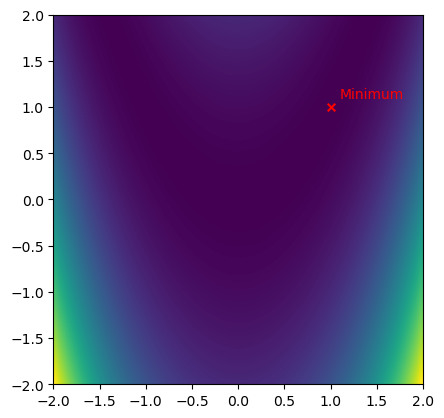
The rosenbrock function’s minimum is zero at the coordinate x=1 in all dimensions. We’ll use 2D as an example, because it is easily plottable, but all of the optimizers in prysm work on even extremely high dimensional problems quickly.

import numpy as np

from matplotlib import pyplot as plt

from prysm.x.optym import RMSProp

# make a view of the cost function topology
x = np.linspace(-2,2,100)
y = np.linspace(-2,2,100)
xx, yy = np.meshgrid(x, y)
z = np.zeros_like(xx)
v = np.zeros(2)
for i in range(z.shape[0]):
    for j in range(z.shape[1]):
        v[0] = xx[i,j]
        v[1] = yy[i,j]
        z[i,j] = rosen(v)

plt.imshow(z, origin='lower', extent=[x.min(), x.max(), y.min(), y.max()], interpolation='lanczos')
plt.scatter([1], [1], marker='x', s=30, c='r')
plt.text(1.1,1.1,'Minimum', c='r')

Text(1.1, 1.1, 'Minimum')

To begin optimization, we specify an initial position x0 and initialize the optimizer:

x0 = np.asarray([-1,1], dtype=float)
opt = RMSProp(cost_grad, x0, alpha=2e-1)

With the exception of F77LBFGSB, none of the optimizers make any tests of convergence or divergence, and will iterate infinitely if you ask them to. To iterate, all optimizers simply provide a def step(self): -> (xk, fk, gk) method, which returns the parameter vector at the start of that iteration, the cost \(\mathcal{L}\) at the start of that iteration, and the gradient \(\nabla\) at the start of that iteration. Optimization is as simple as calling step in a loop:

# do 10 iters of optimization
for i in range(10):
    xk, fk, gk = opt.step()
    print(i, fk)

0 4.0
1 76.67729274647716
2 43.92450733687095
3 34.826874524883145
4 2.7713305397249597
5 2.7105957401052505
6 2.693468596170541
7 2.6803262077070555
8 2.6672787996765055
9 2.6536720508522484

To improve ergonomics, optym provides a convenience runN method which returns a generator yielding (xk, fk, gk). If you wish to track the progress of optimization in real-time and plot the optimizer trajectory, tqdm integrates well:

from prysm.x.optym import runN
from tqdm import tqdm

# re-initialize, throwing away progress
opt = RMSProp(cost_grad, x0, alpha=2e-2)
max_iter = 5_000
f_hist = []
x_hist = []
with tqdm(total=max_iter) as pbar:
    for xk, fk, gk in runN(opt, max_iter):
        fkf = float(fk)  # if you use cupy as a backend, this will be a size 1 vector
        f_hist.append(fkf)
        x_hist.append(xk)
        pbar.set_description(f'Current cost: {fkf:.3g}', refresh=False)
        pbar.update(1)

Current cost: 0.0878: 100%|██████████| 5000/5000 [00:00<00:00, 24446.63it/s]

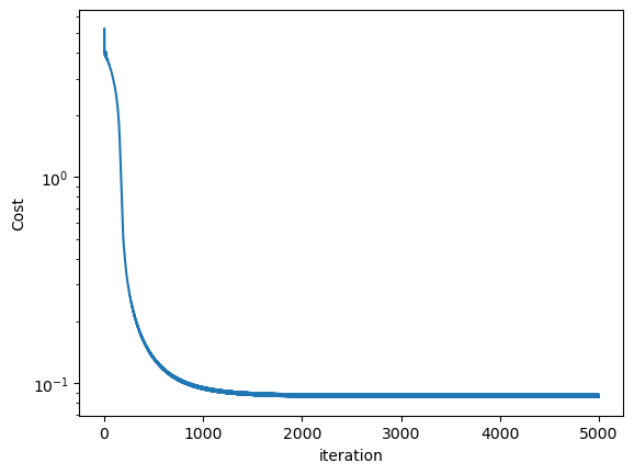
Now we can plot the cost history:

plt.semilogy(f_hist)
plt.gca().set(ylabel='Cost', xlabel='iteration')

[Text(0, 0.5, 'Cost'), Text(0.5, 0, 'iteration')]

Governed Optimization

Fixed-count loops are useful when you are experimenting, but production optimization usually wants a reusable stopping rule. optym calls these stopping rules governors. A governor observes the completed step records from an optimizer and decides whether the run should continue.

The run_until runner keeps the optimizer’s simple step() contract intact, but owns the stop logic. Here we switch to Adam for a less hand-tuned run of the same Rosenbrock problem, then stop when any governor says the run is finished.

from prysm.x.optym import (
    Adam,
    AnyGovernor,
    FunctionTolerance,
    GradientTolerance,
    MaxIterations,
    StepTolerance,
    plot_convergence,
    run_until,
)

opt = Adam(cost_grad, x0, alpha=1e-2)
governor = AnyGovernor([
    GradientTolerance(1e-4),
    FunctionTolerance(1e-12),
    StepTolerance(1e-12),
    MaxIterations(10_000),
])

result = run_until(opt, governor)
result.message, result.nit, result.x

('gradient tolerance reached', 1213, array([0.99987024, 0.99974001]))

The result contains the final parameter vector and every StepRecord observed by the governors. That history can be sent straight to plot_convergence to inspect the objective and gradient norm versus iteration.

fig, ax = plot_convergence(result, quantities=('f', 'g_norm'), yscale='log')

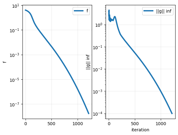
We can see that the optimizer stopped making improvement after iteration 1000 or so. Lets look at the trajectory it followed to see if we can get a clue why:

plt.figure()
xh = np.asarray(x_hist)
plt.imshow(z, origin='lower', extent=[x.min(), x.max(), y.min(), y.max()], interpolation='lanczos')
plt.scatter([1], [1], marker='x', s=30, c='r')
plt.plot(*xh.T, c='#FF5555') # transpose to get (x,y) on the front dimension, then unpack because plot wants plot(x, y)
plt.text(1.1,1.1,'Minimum', c='r')

Text(1.1, 1.1, 'Minimum')

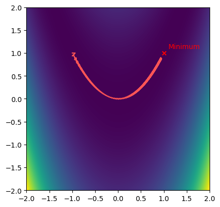
We can see that the optimizer was oscillating from the zig-zag pattern it was making, but was making progress. Generally oscillation is the result of too much gain, so lets try detuning alpha after 1000 iterations:

# copy-paste, except for last line
opt = RMSProp(cost_grad, x0, alpha=2e-2)
max_iter = 5_000
f_hist = []
x_hist = []
with tqdm(total=max_iter) as pbar:
    for xk, fk, gk in runN(opt, max_iter):
        fkf = float(fk)  # if you use cupy as a backend, this will be a size 1 vector
        f_hist.append(fkf)
        x_hist.append(xk)
        pbar.set_description(f'Current cost: {fkf:.3g}', refresh=False)
        pbar.update(1)

        if opt.iter == 1000:
            opt.alpha /= 10

Current cost: 0.000902: 100%|██████████| 5000/5000 [00:00<00:00, 28275.05it/s]

fig, axs = plt.subplots(ncols=2, figsize=(8,4))
axs[0].semilogy(f_hist)
axs[0].set(ylabel='Cost', xlabel='iteration')

xh = np.asarray(x_hist)
axs[1].imshow(z, origin='lower', extent=[x.min(), x.max(), y.min(), y.max()], interpolation='lanczos')
axs[1].scatter([1], [1], marker='x', s=30, c='r')
axs[1].plot(*xh.T, c='#FF5555') # transpose to get (x,y) on the front dimension, then unpack because plot wants plot(x, y)

[<matplotlib.lines.Line2D at 0x72efdc31da90>]

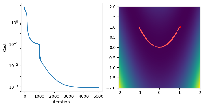
We can see that detuning the gain took us much closer to the minimum, but we actually could have detuned it much earlier! And the oscillation is not completely gone. These all suggest further tuning of RMSProp would lead to better performance on this problem, which is outside the scope of this tutorial. For those wishing to explore this further, yet another dimension is that most of the optimizers store some sort of internal state. Most all optimizers have smooth behavior if you change alpha, but you may find the state is somewhat poisoned by the past, and creating a new optimizer with different hyperparameters, initialized at the current best xk does better. So much to explore!

Wrap-Up

In this tutorial, we learned how to use x/optym to perform gradient-based optimization. We used a difficult toy problem to exercise the machinery, tried both fixed-count loops and governed runs, and began exploring the possibilities afforded by adjusting optimizer hyperparameters while the optimizer is working. With this information, you should be prepared to create your own cost function and gradient and use these nonlinear optimization techniques to solve problems.