Radiometrically Correct Modeling
This notebook will show how to condition inputs to prysm such that they preserve radiometry. By doing so, the user is able to model not only the morphology of the diffraction image but also the noise properties and fundamental scaling. We’ll start with a circular aperture and show that this extends to others as well.
[1]:
import numpy as np

from prysm.coordinates import make_xy_grid, cart_to_polar
from prysm.geometry import truecircle, circle # anti-aliased, but circle would be fine too
from prysm.fttools import pad2d, mdft
from prysm.propagation import focus

from matplotlib import pyplot as plt
First we show a simple PSF model of a diffraction limited point spread function for a circular aperture:
[2]:
x, y = make_xy_grid(256, diameter=2)
r, t = cart_to_polar(x, y)
aperture = circle(1, r)
inc_psf = abs(focus(aperture, Q=2)) ** 2
inc_psf.sum(), inc_psf.max()
[2]:
(13482328063.999996, 2645147761.0)
With no effort on the part of the user, prysm makes no attempt to scale outputs of operations in any physically meaningful way. The focus function is an FFT propagation, and most FFT implementations (including the numpy one used here) do not divide the forward FFT by N, but do divide the reverse FFT by N, such that ifft(fft(x)) ~= x. If we care about radiometry, we either would like the PSF to sum to 1, or for the peak of a diffraction limited PSF to be 1. The latter simply requires dividing
the aperture by its sum:
[3]:
aperture2 = aperture / aperture.sum()
inc_psf = abs(focus(aperture2, Q=2)) ** 2
inc_psf.sum(), inc_psf.max()
[3]:
(5.097003752600571, 1.0)
To achieve the former, we simply need to make the propagation satisfy Parseval’s theorem and make the aperture sum to 1. We can actually achieve better efficiency by scaling the aperture, such that scaling the output is unnecessary. By preconditioning the input, we can make FFT operating on the input satisfy Parseval’s theorem. The aperture is an amplitude, so it requires scaling by \(\sqrt{N}\) in addition to a similarly square-rooted change to what we did to get a peak of 1. A minor
complication is that the padding used to achieve Q=2 increases \(N\), so we’ll pre-pad:
[4]:
aperture3 = pad2d(aperture, Q=2)
aperture3 = aperture3 / (np.sqrt(aperture3.sum()) * np.sqrt(aperture3.size))
inc_psf = abs(focus(aperture3, Q=1)) ** 2
inc_psf.sum(), inc_psf.max()
[4]:
(1.0, 0.19619369506835938)
The fixed sampling propagation requires a brief detour into the algorithm details to understand radiometric scaling. First we define \(\hat{f}\) the fourier transform of \(f\):
This is a continuous symbology. The Discrete Fourier transform (DFT) is defined as:
where \(k, n\) are the output and input sample numbers, and \(K, N\) are the total number of output and input samples. Because there is no normalization, as \(N\) increases, the magnitude of \(\hat{f}\) will grow. The same is not true for a growth in \(K\).
Further, we can see that the kernel of exp is precisely \(\cos - i \sin\), which is the continuous Fourier mode. The only difference between the definition of the FT and the DFT is in the discrete sum replacing an integral, and scaling of the kernel into the Nyquist bounds of \([-f_s/2, f_s]\), with \(f_s = 1 / dx\).
When we take a zoomed DFT as done in focus_fixed_sampling, the value of \(N\) is unchanged but the value of \(K\) and the spatial frequency interval \(d\nu\) are changed.
We can think of the outputs we may desire:
Overlapping zoomed DFT and FFT samples to have the same magnitude
The zoomed DFT output not to violate Parseval’s theorem
The DC frequency bin to have a value of 1.
A zoomed DFT into the core of a PSF that is re-transformed to the aperture’s domain in pupil space to lose as little energy as possible.
Item (2) is not possible in general. For a non bandlimited function such as the hard edged circular or square aperture, the PSF is an “infinite impulse response” (IIR) and computing it over a bandpass that does not extend to \(f_s\) necessarily discards part of the signal and loses energy. For bandlimited functions, (2) may be achieved. Item (3) is always possible, and with no effort expended (1) is also achieved. (4) is subject to the same provisions as mentioned for IIR systems, but can be implemented if we assume our functions are bandlimited, or the user accepts the loss of energy inherent in discarding some of the outer regions of the PSF.
The zoomed DFT (or matrix triple product or matrix DFT) implemented in prysm is “unnormalized” in the same way the FFT backend is. Within cases where the zoomed DFT could have been computed as a combination of FFT and cropping operations, zoomed DFT ~= FFT, up to floating point rounding. Observe:
[5]:
# 1) zoomed DFT ~= FFT
# note, mdft.dft2 is used for the sake of clear example, but propagation.focus_fixed_sampling
# is just a different interface to this
inc_psf = abs(focus(aperture2, Q=2)) ** 2
print(inc_psf.sum(), inc_psf.max())

inc_psf2 = mdft.dft2(aperture2, 2, 512)
inc_psf2 = abs(inc_psf2)**2
print(inc_psf2.sum(), inc_psf2.max())
5.097003752600571 1.0
5.097003752600583 1.0000000000000044
Note that these agree to all but the last two digits. We can see that if we “crop” into the zoomed DFT by computing fewer samples, our peak answer does not change and the sum is nearly the same (since the region of the PSF distant to the core carries very little energy):
[6]:
inc_psf2 = mdft.dft2(aperture2, 2, 128)
inc_psf2 = abs(inc_psf2)**2
print(inc_psf2.sum(), inc_psf2.max())
5.068251173139342 1.0000000000000044
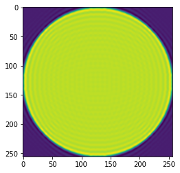
In this case, we lost about 0.03/5 ~= 0.6% of the energy. If we go back to the pupil,
[7]:
# for the magic number 4, consider that the Q=2 FFT would produce 512x512 and the computed region
# is 128x128

field = mdft.dft2(aperture2, 2, 128)  # note that we are propagating the e field back to the pupil, not the PSF
aperture_clone = mdft.idft2(field, 4, 256)
aperture_clone = aperture_clone.real / field.size / 4 / 4
plt.imshow(aperture_clone)
[7]:
<matplotlib.image.AxesImage at 0x7f9fd0d17f40>
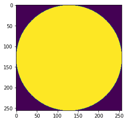
[8]:
plt.imshow(aperture2)
[8]:
<matplotlib.image.AxesImage at 0x7f9fd0417880>
[9]:
print(aperture2.max(), aperture2.sum())
print(aperture_clone.max(), aperture_clone.sum())
1.9443526277925766e-05 1.0000000000000002
3.3427233106365233e-10 1.5254221904110318e-05
We can see that at first blush, the process does not duplicate itself. This is because of the IIR nature of the PSF. The destruction of high frequencies via the crop implicit in computing a \(Q=2\) field with \(< 2*N\) samples results in spatial domain ringing. This ringing has resulted in the pupil being 0.0003 dimmer in its total energy, likely due to a small amount of energy cast outside the computational window. There is also a ~10% overshoot in the maximum value.
A related phenomenon will occur if you compute a domain that goes beyond \(f_s/2\), since the Dirichlet aliases will be visible in the field variable before inverse transformation, and the Fourier transform of a signal and a noninteger number of its aliases is not the same as the Fourier transform of the signal itself.
In Summary
prysm’s FFT propagations are not normalized. Scaling input amplitudes by \(\sum(f)\) or by \(\sqrt{N}\sqrt{\sum(f)}\) will produce focused fields which have peaks of 1, or sums of 1. The zoomed DFT computations follow precisely the same rules as the FFT computations, except for some caveats about non-bandlimited functions and energy loss.