Notable Telescope Apertures
This notebook will show how to use prysm to paint the apertures of notable telescopes. Further modeling of these observatories will not be given here, and requries additional data (e.g., OPD maps or coefficients, masks) not widely available. It is assumed the user sufficiently understands the components used to not require explanation of details. All parameters are based on publically shown values and may be imprecise. If you are a member of the science or engineering team for these systems, you should check all parameters against internal values.
Most apertures include the steps to repeat this synthesis for any similar aperture, and do not jump directly to the solution. They all conclude with a mask and a figure showing the fully composited aperture.
Links jump to telescopes:
[1]:
import numpy as np

from prysm.coordinates import make_xy_grid, cart_to_polar
from prysm.geometry import spider, circle, offset_circle
from prysm.segmented import CompositeHexagonalAperture

from matplotlib import pyplot as plt
HST
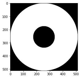
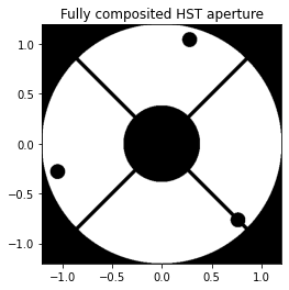
HST has a primary mirror of diameter 2.4 m with 32% linear obscuration, and four spiders of 38 mm diameter rotated 45\(^\circ\) from the cardinal axes. There are an additional three small circular obscurations from pads used to secure the primary mirror. The pads are 90% of the way to the edge of the mirror at ccw angles w.r.t. the x axis of -45, -165, and +75 degrees and have each a diameter of 150 mm.
[2]:
x, y = make_xy_grid(512, diameter=2.4)
r, t = cart_to_polar(x, y)

pm_od = circle(2.4/2, r)
pm_id = circle(2.4/2*.32, r)
mask = pm_od ^ pm_id # or pm_od & ~pm_id
plt.imshow(mask, cmap='gray')
[2]:
<matplotlib.image.AxesImage at 0x7f07b45c6430>
After shading the primary, we now compute the spider and pad obscurations:
[3]:
spider_ = spider(4, 0.038, x, y, 45)
pads_r = 0.90*2.4/2
pad_angles = [np.radians(a) for a in [-45, -165, 75]]
pad_centers = [(pads_r*np.cos(a), pads_r*np.sin(a)) for a in pad_angles]
pads = [offset_circle(.075, x, y, c) for c in pad_centers]

# pads before this point is a list of the points INSIDE each circle.
# logical or, |, below produces a mask of "pixels inside ANY circle"
# these are an obscuration, so we invert it with ~
pads = (pads[0]|pads[1]|pads[2])
hst_pupil = mask & spider_ & ~pads
plt.imshow(hst_pupil, origin='lower', cmap='gray', extent=[x.min(), x.max(), y.min(), y.max()])
plt.title('Fully composited HST aperture')
[3]:
Text(0.5, 1.0, 'Fully composited HST aperture')
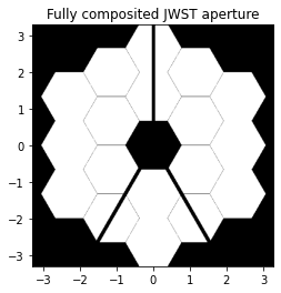
JWST
JWST is a 2-ring segmented hexagonal design. The central segment is missing, and there is a upside-down “Y” strut system to hold the secondary. The segments are 1.32 m flat-to-flat, with 7 mm airgaps between. We first paint the hexagons:
[4]:
x, y = make_xy_grid(512, diameter=6.6)

cha = CompositeHexagonalAperture(x,y,2,1.32,0.007,exclude=(0,))

plt.imshow(cha.amp, origin='lower', cmap='gray', extent=[x.min(), x.max(), y.min(), y.max()])
[4]:
<matplotlib.image.AxesImage at 0x7f07b4dadfd0>
And create the secondary struts, adding them to the mask:
[5]:
m1 = spider(1, .1, x, y, rotation=-120)
m2 = spider(1, .1, x, y, rotation=-60)
m3 = spider(1, .1, x, y, rotation=90)
spider_ = m1&m2&m3
plt.imshow(cha.amp&spider_, origin='lower', cmap='gray', extent=[x.min(), x.max(), y.min(), y.max()])
plt.title('Fully composited JWST aperture')
[5]:
Text(0.5, 1.0, 'Fully composited JWST aperture')
TMT
TMT is a hexagonally tiled aperture with 1.44 m segments (diameter, not flat-to-flat) and only 2.5 mm gaps. The gaps cannot be drawn properly except on a very fine grid (30M/2.5mm ~= 12K array to get 1 sample per gap). 13 rings are required to shade the entire aperture. The first step in defining the aperture is to indicate which segment has which ID from prysm (which are deterministic) and mark the ones missing from the observatory for exclusion:
[6]:
x, y = make_xy_grid(1024, diameter=30)
r, t = cart_to_polar(x, y)

flat_to_flat_to_vertex_vertex = 2 / np.sqrt(3)
vtov_to_flat_to_flat = 1 / flat_to_flat_to_vertex_vertex

segdiam = vtov_to_flat_to_flat * 1.44
cha = CompositeHexagonalAperture(x,y,13,segdiam,0.0025)

fig, ax = plt.subplots(figsize=(15,15))
ax.imshow(cha.amp, origin='lower', cmap='gray', extent=[x.min(), x.max(), y.min(), y.max()])
for center, id_ in zip(cha.all_centers, cha.segment_ids):
    plt.text(*center, id_, ha='center', va='center')
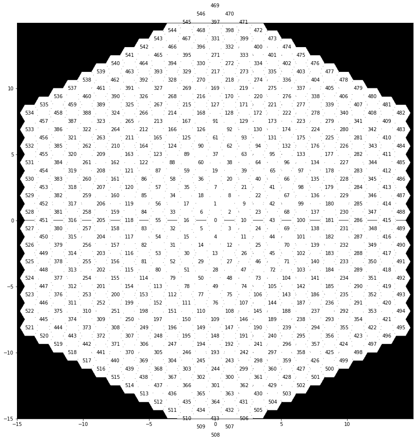
The inner ring and center segment should be excluded, and only 6 segments exist per horizontal side, nor should the most extreme “columns” be present. The topmost segments are also not present. Let’s start with this as an exclusion list:
[7]:
exclude = [
    0, 1, 2, 3, 4, 5, 6, # center
    469, 470, 508, 509, 507, 510, 506, 545,
    471, 511, 505, 544, 472, 397, 433, 546, # top, bottom
    534, 533, 532, 531, 521, 522, 523, 524, # left edge
    482, 483, 484, 485, 495, 494, 493, 492, # right edge
]

cha = CompositeHexagonalAperture(x,y,13,segdiam,0.0025, exclude=exclude)
fig, ax = plt.subplots(figsize=(15,15))
ax.imshow(cha.amp, origin='lower', cmap='gray', extent=[x.min(), x.max(), y.min(), y.max()])
for center, id_ in zip(cha.all_centers, cha.segment_ids):
    plt.text(*center, id_, ha='center', va='center')
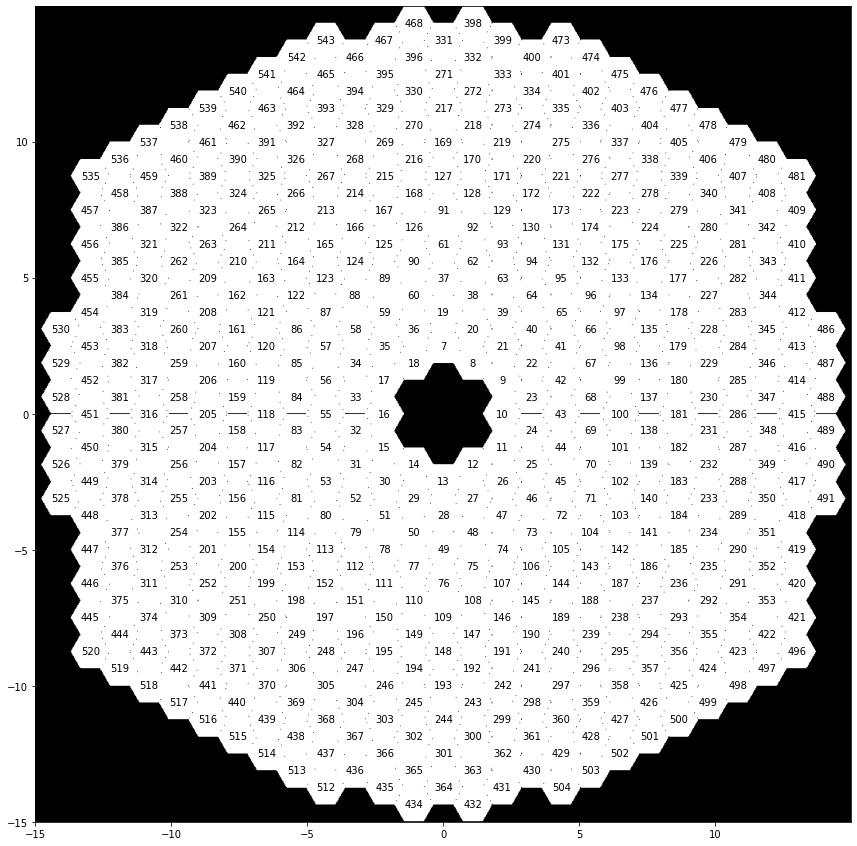
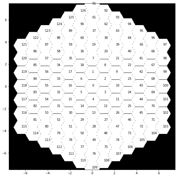
Next we can see that the diagonal “corners” are too large. With the exclusion list below, we can create a TMT pupil, excepting struts and SM obscuration, in only two lines of code.
[8]:
exclude = [
    0, 1, 2, 3, 4, 5, 6, # center
    469, 470, 508, 509, 507, 510, 506, 545,
    471, 511, 505, 544, 472, 397, 433, 546, # top, bottom
    534, 533, 532, 531, 521, 522, 523, 524, # left edge
    482, 483, 484, 485, 495, 494, 493, 492, # right edge
    457, 535, 445, 520, 481, 409, 421, 496, # corners
    536, 537, 479, 480, 497, 498, 519, 518, # next 'diagonal' from corners
]

cha = CompositeHexagonalAperture(x,y,13,segdiam,0.0025, exclude=exclude)
fig, ax = plt.subplots(figsize=(15,15))
ax.imshow(cha.amp, origin='lower', cmap='gray', extent=[x.min(), x.max(), y.min(), y.max()])
[8]:
<matplotlib.image.AxesImage at 0x7f07b48ebd00>
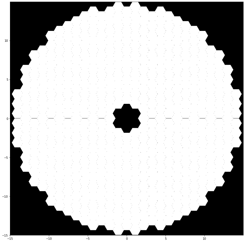
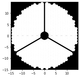
The TMT secondary obscuration is of 3.65 m diameter, we add it and struts of 50 cm diameter that are equiangular:
[9]:
spider_ = spider(3, .5, x, y, rotation=90)
sm_obs = ~circle(3.65/2, r)
plt.imshow(cha.amp&spider_&sm_obs, origin='lower', cmap='gray', extent=[x.min(), x.max(), y.min(), y.max()])
[9]:
<matplotlib.image.AxesImage at 0x7f07b4c34f10>
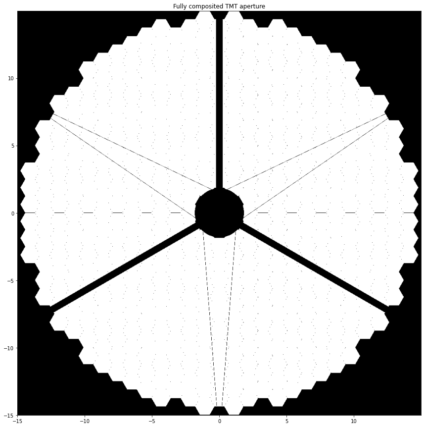
Last of all are the six cables, of 20 mm diameter. These are a bit tricky, but they have a meeting point at 90% the radius of the SM obscuration. We will form them similar to the JWST and LUVOIR-A spiders, by shifting the coordinate grid and specifying the angle. The angles are about 10\(^\circ\) from the radial normal.
[10]:
# first cable bundle
r_offset = 3.65/2*.8
center_angle = np.radians(90)
center_c1 = (np.cos(center_angle) * r_offset, np.sin(center_angle) * r_offset)
cable1 = spider(1, 0.02, x, y, rotation=25.5, center=center_c1)
cable2 = spider(1, 0.02, x, y, rotation=180-25.5, center=center_c1)

center_angle = np.radians(-30)
center_c1 = (np.cos(center_angle) * r_offset, np.sin(center_angle) * r_offset)
cable3 = spider(1, 0.02, x, y, rotation=34.5, center=center_c1)
cable4 = spider(1, 0.02, x, y, rotation=-90-4.5, center=center_c1)

center_angle = np.radians(210)
center_c1 = (np.cos(center_angle) * r_offset, np.sin(center_angle) * r_offset)
cable5 = spider(1, 0.02, x, y, rotation=180-34.5, center=center_c1)
cable6 = spider(1, 0.02, x, y, rotation=-90+4.5, center=center_c1)

cables = cable1&cable2&cable3&cable4&cable5&cable6
fig, ax = plt.subplots(figsize=(15,15))
ax.imshow(cha.amp&spider_&sm_obs&cables, origin='lower', cmap='gray', extent=[x.min(), x.max(), y.min(), y.max()])
ax.set_title('Fully composited TMT aperture')
[10]:
Text(0.5, 1.0, 'Fully composited TMT aperture')
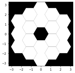
LUVOIR-A
LUVOIR-A (as of the 2018 new design) contains 120 hexagonal segments of flat-to-flat dimension 1.223 m. Only the central segment is missing. The strut design is essentially the same as JWST. The first step in defining the aperture is to indicate which segment has which ID from prysm (which are deterministic) and mark the ones missing from the observatory for exclusion:
[11]:
x, y = make_xy_grid(512, diameter=15)

cha = CompositeHexagonalAperture(x,y,6,1.223,0.007)
fig, ax = plt.subplots(figsize=(10,10))
ax.imshow(cha.amp, origin='lower', cmap='gray', extent=[x.min(), x.max(), y.min(), y.max()])
for center, id_ in zip(cha.all_centers, cha.segment_ids):
    plt.text(*center, id_)
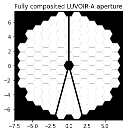
Note that we have discarded all of the other information from the composition process, which will be identical to the previous invocation. We now add the spider, pretty much the same as JWST:
[12]:
exclude = [
    0,
    91,
    109,
    97,
    103,
    115,
    121
]

cha = CompositeHexagonalAperture(x,y,6,1.223,0.007, exclude=exclude)

m1 = spider(1, .2, x, y, rotation=-105)
m2 = spider(1, .2, x, y, rotation=-75)
m3 = spider(1, .2, x, y, rotation=90)
spider_ = m1&m2&m3
plt.imshow(cha.amp&spider_, origin='lower', cmap='gray', extent=[x.min(), x.max(), y.min(), y.max()])
plt.title('Fully composited LUVOIR-A aperture')
[12]:
Text(0.5, 1.0, 'Fully composited LUVOIR-A aperture')
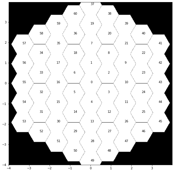
LUVOIR-B
LUVOIR-B is a smaller, unobscured co-design to LUVOIR-A. We follow a similar two-step shading process to find which segment IDs must be excluded:
[13]:
x, y = make_xy_grid(512, diameter=8)

cha = CompositeHexagonalAperture(x,y,4,.955,.007)

fig, ax = plt.subplots(figsize=(10,10))
ax.imshow(cha.amp, origin='lower', cmap='gray', extent=[x.min(), x.max(), y.min(), y.max()])
for center, id_ in zip(cha.all_centers, cha.segment_ids):
    plt.text(*center, id_)
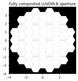
[14]:
exclude = [
    37,
    41,
    45,
    49,
    53,
    57
]

cha = CompositeHexagonalAperture(x,y,4,.955,.007, exclude=exclude)


plt.imshow(cha.amp, origin='lower', cmap='gray', extent=[x.min(), x.max(), y.min(), y.max()])
plt.title('Fully composited LUVOIR-B aperture')
[14]:
Text(0.5, 1.0, 'Fully composited LUVOIR-B aperture')
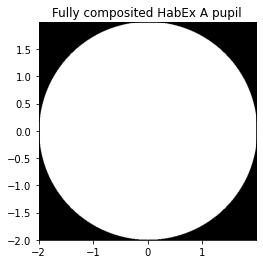
HabEx-A
Habex architecture A is a 4m unobscured system, which is extremely simple to model:
[15]:
x, y = make_xy_grid(512, diameter=4)
r, t = cart_to_polar(x, y)
mask = circle(2, r)

plt.imshow(mask, origin='lower', cmap='gray', extent=[x.min(), x.max(), y.min(), y.max()])
plt.title('Fully composited HabEx A pupil')
[15]:
Text(0.5, 1.0, 'Fully composited HabEx A pupil')
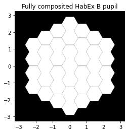
HabEx-B
Habex architecture B is an unobscured pupil of 6.5 m diameter based on a 3-ring fully populated hexagonal composition
[16]:
x, y = make_xy_grid(512, diameter=6.5)

cha = CompositeHexagonalAperture(x,y,3,.825,0.007)

plt.imshow(cha.amp, origin='lower', cmap='gray', extent=[x.min(), x.max(), y.min(), y.max()])
plt.title('Fully composited HabEx B pupil')
[16]:
Text(0.5, 1.0, 'Fully composited HabEx B pupil')