Interferograms
Prysm offers rich features for analysis of interferometric data. Interferogram objects are conceptually similar to Pupils and both inherit from the same base class, as they both have to do with optical phase. The construction of an Interferogram requires only a few parameters:
[1]:
import numpy as np
from prysm import Interferogram
x = y = np.arange(129)
z = np.random.uniform((128,128))
interf = Interferogram(phase=z, intensity=None, x=x, y=y, scale='mm', phase_unit='nm', meta={'wavelength': 632.8e-9})
Notable are the scale, and phase unit, which define the x, y, and z units. Any SI unit is accepted as well as angstroms. Imperial units not accepted. meta is a dictionary to store metadata. For several interferogram methods to work, the wavelength must be present in meters. This departure from prysm’s convention of preferred units is used to maintain compatability with Zygo dat files. Interferograms are usually created from such files:
[2]:
from prysm import sample_files

interf = Interferogram.from_zygo_dat(sample_files('dat'))
and both the dat and datx format from Zygo are supported. Dat carries no dependencies, while datx requries the installation of h5py. In addition to properties inherited from the OpticalPhase class (pv, rms, Sa, std), Interferograms have a PVr property, for C. Evan’s Robust PV metric, and dropout_percentage property, which gives the percentage of NaN values within the phase array. These NaNs may be filled,
[3]:
interf.fill(_with=0)
[3]:
<prysm.interferogram.Interferogram at 0x7fe9081d44e0>
with 0 as a default value; only constants are supported. The modification is done in-place and the method returns self. Piston, tip-tilt, and power may be removed:
[4]:
interf.remove_piston().remove_tiptilt().remove_power()
[4]:
<prysm.interferogram.Interferogram at 0x7fe9081d44e0>
again done in-place and returning self, so methods can be chained. You should remove these terms (or, indeed do anything with Zernikes) before filling NaNs. One line convenience wrappers exist:
[5]:
interf.remove_piston_tiptilt()
interf.remove_piston_tiptilt_power()
[5]:
<prysm.interferogram.Interferogram at 0x7fe9081d44e0>
spikes may also be clipped,
[6]:
interf.spike_clip(nsigma=3) # default is 3
[6]:
<prysm.interferogram.Interferogram at 0x7fe9081d44e0>
setting points with a value more than nsigma standard deviations from the mean to NaN.
If the data did not have a lateral calibration baked into it, you can provide one in prysm,
[7]:
# this is not going to do what you want if your data is already calibrated.
interf.latcal(plate_scale=0.1, unit='mm')
[7]:
<prysm.interferogram.Interferogram at 0x7fe9081d44e0>
Masks may be applied:
[8]:
your_mask = np.ones(interf.phase.shape)
interf.mask(your_mask)
interf.mask('circle', diameter=4)  # 4 <spatial_unit> diameter circle
[8]:
<prysm.interferogram.Interferogram at 0x7fe9081d44e0>
The truecircle mask should not be used on interferometric data. the phase is deleted (replaced with NaN) wherever the mask is equal to zero.
Interferograms may be cropped, deleting empty (NaN) regions around a measurment;
[9]:
interf.crop()
[9]:
<prysm.interferogram.Interferogram at 0x7fe9081d44e0>
Convenience properties are provided for data size,
[10]:
interf.shape, interf.size, interf.diameter_x, interf.diameter_y, interf.diameter, interf.semidiameter
[10]:
((339, 339),
 114921,
 3.9858380492660217,
 3.9858380492660217,
 3.9858380492660217,
 1.9929190246330108)
shape and size mirrors the underlying interf.phase ndarray. The x and y diameters are in units of interf.spatial_unit and diameter is the greater of the two.
The two dimensional Power Spectral Density (PSD) may be computed. The data may not contain NaNs, and piston tip and tilt should be removed prior. A 2D Welch window is used for circular data and a 2D Hanning window for rectangular data, so there is no need for concern about zero values creating a discontinuity at the edge of circular or other nonrectangular apertures.
[11]:
interf.crop().remove_piston_tiptilt_power().fill()
ux, uy, psd = interf.psd()
several slices are also available,
[12]:
psd_dict = interf.psd_slices(x=True, y=True, azavg=True, azmin=True, azmax=True)
ux, psd_x = psd_dict['x']
uy, psd_y = psd_dict['y']
ur, psd_r = psd_dict['azavg']
and the PSD may be plotted,
[13]:
interf.plot_psd2d(axlim=1, interp_method='lanczos', fig=None, ax=None)
interf.plot_psd_slices(xlim=(1e0,1e3), ylim=(1e-7,1e2), fig=None, ax=None)
[13]:
(<Figure size 640x480 with 1 Axes>,
 <matplotlib.axes._subplots.AxesSubplot at 0x7fe8dd9d1160>)
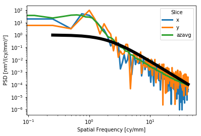
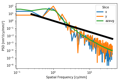
For the slices plot, a Lorentzian or power law model may be plotted alongside the data for e.g. visual verification of a requirement:
[14]:
interf.plot_psd_slices(a=1,b=2,c=3)
interf.plot_psd_slices(a=1,b=1.5)
[14]:
(<Figure size 432x288 with 1 Axes>,
 <matplotlib.axes._subplots.AxesSubplot at 0x7fe8dd9ae2e8>)
A bandlimited RMS value derived from the 2D PSD may also be evaluated,
[15]:
interf.bandlimited_rms(wllow=1, wlhigh=10, flow=1, fhigh=10)
[15]:
9.42102378723147
only one of wavelength (wl; spatial period) or frequency (f) should be provided. f will clobber wavelength.
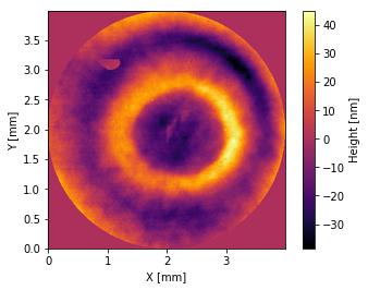
[16]:
interf.plot2d()
[16]:
(<Figure size 432x288 with 2 Axes>,
 <matplotlib.axes._subplots.AxesSubplot at 0x7fe8dd485e80>)