Radiometrically Correct Modeling#
This notebook will show how to condition inputs to prysm such that they preserve radiometry. By doing so, the user is able to model not only the morphology of the diffraction image but also the noise properties and fundamental scaling. We’ll start with a circular aperture and show that this extends to others as well.
[1]:
import numpy as np

from prysm.coordinates import make_xy_grid, cart_to_polar
from prysm.geometry import circle
from prysm.fttools import pad2d, mdft
from prysm.propagation import focus

from matplotlib import pyplot as plt
First we show a simple PSF model of a diffraction limited point spread function for a circular aperture:
[2]:
x, y = make_xy_grid(256, diameter=2)
r, t = cart_to_polar(x, y)
aperture = circle(1, r)
inc_psf = abs(focus(aperture, Q=2)) ** 2
inc_psf.sum(), inc_psf.max()
[2]:
(51430.999999999985, 10090.437931060791)
The focus function is an FFT propagation, and uses the norm='unitary' scaling, which preserves Parseval’s theorem. The satisfaction is in terms of complex E-field, but we are interested in unit intensity, so we must also divide by the square root of the sum of the aperture if we’d like the result to peak at 1.0:
[3]:
aperture2 = aperture / np.sqrt(aperture.sum())
inc_psf = abs(focus(aperture2, Q=2)) ** 2
inc_psf.sum(), inc_psf.max()
[3]:
(1.0, 0.19619369506835938)
To achieve a peak of one, we need to scale the aperture in a particular way:
[4]:
aperture3 = pad2d(aperture, Q=2)
aperture3 = aperture3 * (2*np.sqrt(aperture.size)/aperture.sum())
inc_psf = abs(focus(aperture3, Q=1)) ** 2
inc_psf.sum(), inc_psf.max()
[4]:
(5.097003752600571, 1.0)
Use of matrix DFTs (and chirp Z transforms) provides equal energy to FFTs, except when performing asymmetric transform pairs (one domain is smaller or larger than the other):
[5]:
# 1) zoomed DFT ~= FFT
# note, mdft.dft2 is used for the sake of clear example, but propagation.focus_fixed_sampling
# is just a different interface to this
inc_psf = abs(focus(aperture2, Q=2)) ** 2
print(inc_psf.sum(), inc_psf.max())

inc_psf2 = mdft.dft2(aperture2, 2, 512)
inc_psf2 = abs(inc_psf2)**2
print(inc_psf2.sum(), inc_psf2.max())
1.0 0.19619369506835938
1.0000000000000027 0.19619369506836032
Note that these agree to all but the last two digits. We can see that if we “crop” into the zoomed DFT by computing fewer samples, our peak answer does not change and the sum is nearly the same (since the region of the PSF distant to the core carries very little energy):
[6]:
inc_psf2 = mdft.dft2(aperture2, 2, 128)
inc_psf2 = abs(inc_psf2)**2
print(inc_psf2.sum(), inc_psf2.max())
0.9943589251927554 0.19619369506836032
In this case, we lost about 0.03/5 ~= 0.6% of the energy. If we go back to the pupil, a factor of 2 scaling will be needed due to the 2X crop used in the focal plane; 128 = 0.5 * 256, or 256 = 128 * 2
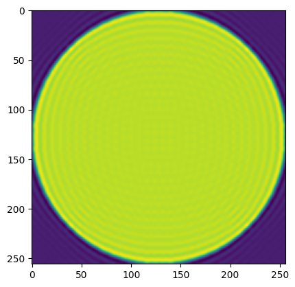
[7]:
field = mdft.dft2(aperture2, 2, 128)  # note that we are propagating the e field back to the pupil, not the PSF
aperture_clone = mdft.idft2(field, 4, 256)
aperture_clone = aperture_clone.real * 2
plt.imshow(aperture_clone)
[7]:
<matplotlib.image.AxesImage at 0x7ffa18398fd0>
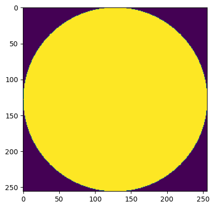
[8]:
plt.imshow(aperture2)
[8]:
<matplotlib.image.AxesImage at 0x7ffa182fe5b0>
[9]:
print(aperture2.max(), aperture2.sum())
print(aperture_clone.max(), aperture_clone.sum())
0.004409481406914623 226.7840382390259
0.009936257562730526 453.43231752383264
We can see that at first blush, the process does not duplicate itself. This is because of the IIR nature of the PSF. The destruction of high frequencies via the crop implicit in computing a \(Q=2\) field with \(< 2*N\) samples results in spatial domain ringing. This ringing has resulted in the pupil being 0.0003 dimmer in its total energy, likely due to a small amount of energy cast outside the computational window. There is also a ~10% overshoot in the maximum value.
A related phenomenon will occur if you compute a domain that goes beyond \(f_s/2\), since the Dirichlet aliases will be visible in the field variable before inverse transformation, and the Fourier transform of a signal and a noninteger number of its aliases is not the same as the Fourier transform of the signal itself.
In Summary#
prysm’s propagations are normalized such that,
If you desire a sum of 1, scale \(f = f / \sqrt{\sum f}\)
If you desire a peak of one, scale \(f = f \cdot \left( Q\cdot \sqrt{\frac{N}{\sum f}} \right)\)