Radiometrically Correct Modeling

This notebook will show how to condition inputs to prysm such that they preserve radiometry. By doing so, the user is able to model not only the morphology of the diffraction image but also the noise properties and fundamental scaling. We’ll start with a circular aperture and show that this extends to others as well.

import numpy as np

from prysm.coordinates import make_xy_grid, cart_to_polar
from prysm.geometry import circle
from prysm.fttools import pad2d
from prysm.propagation import focus, focus_dft, prepare_executor, unfocus_dft

from matplotlib import pyplot as plt

First we show a simple PSF model of a diffraction limited point spread function for a circular aperture:

x, y = make_xy_grid(256, diameter=2)
r, t = cart_to_polar(x, y)
dx = x[0,1] - x[0,0]
aperture = circle(1, r)
inc_psf = abs(focus(aperture, Q=2)) ** 2
print('sum', inc_psf.sum(), 'max', inc_psf.max())

sum 51430.999999999985 max 10090.437931060791

The focus function is an FFT propagation, and uses the norm='ortho' scaling, which preserves Parseval’s theorem. The satisfaction is in terms of complex E-field, but we are interested in unit intensity, so we must also divide by the square root of the sum of the aperture if we’d like the result to sum to 1.0. This is equivalent to scaling the aperture to represent one photon in total intensity:

aperture2 = aperture / np.sqrt(aperture.sum())
inc_psf = abs(focus(aperture2, Q=2)) ** 2
print('sum', inc_psf.sum(), 'max', inc_psf.max())

sum 1.0 max 0.19619369506835938

To achieve a peak of one, we need to be aware of the internal normalization done by the norm=ortho convention used by prysm’s FFTs. That convention includes an inner division by \(\sqrt{N\,}\), where N is the number of elements in the array. Since we desire a peak of 1, we can use Parseval’s theorem and simply divide the output array by the sum of the aperture (i.e., the sum of the power in the input beam). Combine that with undoing the normalization done internally by multiplying by \(\sqrt{N\,}\):

padfactor = 2
aperture3 = pad2d(aperture, Q=padfactor)
aperture3 = aperture3 * np.sqrt(aperture3.size)/aperture.sum()
inc_psf = abs(focus(aperture3, Q=1)) ** 2
print('sum', inc_psf.sum(), 'max', inc_psf.max())

sum 5.097003752600571 max 1.0

In this version, we have modified the normalization to increase the power in the aperture by the total number of samples, once again using a square root for energy instead of power. This is a “Stehl” normalization, and the Strehl would be directly evaluate-able using the DC bin of the incoherent PSF if aberrations were introduced.

Use of matrix DFTs (and chirp Z transforms) provides equal energy to FFTs, except when performing asymmetric transform pairs (one domain is smaller or larger than the other):

efl = 10 # F/5
fno = efl/2 # same 2 as diameter in make_xy_grid
wvl = 0.5
# propagation at Q=1 would be 1px/lambda*FNO
q1_dx = fno*wvl

Q = 2
q2_dx = q1_dx / Q

inc_psf = abs(focus(aperture2, Q=2)) ** 2
print('FFT sum', inc_psf.sum(), 'max', inc_psf.max())

executor = prepare_executor(dx, aperture2.shape, q2_dx, 512, wvl, efl)
inc_psf2 = focus_dft(aperture2, executor)
inc_psf2 = abs(inc_psf2)**2
print('MFT sum', inc_psf.sum(), 'max', inc_psf.max())

FFT sum 1.0 max 0.19619369506835938
MFT sum 1.0 max 0.19619369506835938

Note that these agree to all digits. We can see that if we “crop” into the zoomed DFT by computing fewer samples, our peak answer does not change and the sum is nearly the same (since the region of the PSF distant to the core carries very little energy):

executor = prepare_executor(dx, aperture2.shape, q2_dx, 128, wvl, efl)
inc_psf2 = focus_dft(aperture2, executor)
inc_psf2 = abs(inc_psf2)**2
print(inc_psf2.sum(), inc_psf2.max())

0.9943589251927523 0.1961936950683591

In this case, we lost about 0.6% of the energy. This will hold true in the pupil-plane representation if we go back, because each matrix DFT preserves Parseval’s theorem:

executor = prepare_executor(dx, aperture2.shape, q2_dx, 128, wvl, efl)
field = focus_dft(aperture2, executor)  # note that we are propagating the e field back to the pupil, not the PSF
aperture_clone = unfocus_dft(field, executor)
aperture_clone = aperture_clone.real

fig, axs = plt.subplots(ncols=2)
axs[0].imshow(aperture2)
axs[0].set(title=f'True Aperture\nsum: {aperture2.sum():.1f}')

axs[1].imshow(aperture_clone)
axs[1].set(title=f'After Matrix DFT and iDFT\nsum: {aperture_clone.sum():.1f}')

[Text(0.5, 1.0, 'After Matrix DFT and iDFT\nsum: 226.7')]

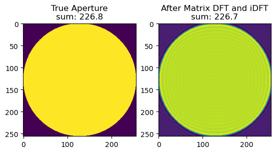
We can see that at first blush, the process does not duplicate itself. This is because of the infinite impulse response nature of the PSF. The destruction of high frequencies via the crop implicit in computing a \(Q=2\) field with \(< 2*N\) samples results in spatial domain ringing. This ringing has resulted in the pupil being minutely dimmer in its total energy, due to the energy that was outside the computed window. There is also a ~10% overshoot in the maximum value.

A related phenomenon will occur if you compute a domain that goes beyond \(f_s/2\), since the Dirichlet aliases will be visible in the field variable before inverse transformation, and the Fourier transform of a signal and a noninteger number of its aliases is not the same as the Fourier transform of the signal itself.

In Summary

prysm’s propagations are normalized such that,

1. If you desire a sum of 1, scale \(f = f \cdot \left(1 / \sqrt{\sum f}\right)\)

2. If you desire a peak of one, scale \(f = f \cdot \left( \sqrt{\text{array size}} /\sum f \right)\)