Ins and Outs of Polynomials#
This document serves as a reference for how prysm is set up to work with polynomials. Much of what differentiates prysm’s API in this area has to do with the fact that it expects the grid to exist at the user level. A fringe benefit is that very nearly all polynomials support analytic derivatives, and all support GPU computation natively.
Bases#
These are the polynomial bases available. Bessel functions are technically special functions, but are placed in the polynomial module for now.
Arbitrary integer orders are available for all modes. If you want to compute the millionth order Zernike term, you can. Bases do not zero, set to NaN, or do anything special when evaluated outside their orthogonal domain. The values of the polynomials are computed as they are.
Sequences and derivatives, fitting, annular and arbitrary domains#
In addition to the various bases, there are four concepts or operations that work independently of the modes.
We’ll start by creating a circular aperture to use for examples:
[1]:
import numpy as np

from prysm.coordinates import make_xy_grid, cart_to_polar
from prysm.geometry import circle

from matplotlib import pyplot as plt

x, y = make_xy_grid(256, diameter=2)
r, t = cart_to_polar(x, y)
mask = ~circle(1,r)  # invert: mask is true outside the circle
Matplotlib is building the font cache; this may take a moment.
Hopkins#
The simplest polynomials are Hopkins’:
for some set of coefficients. The usage of this should not be surprising, for \(W_{131}\), coma one can write:
[2]:
from prysm.polynomials import hopkins
cma = hopkins(1, 3, 1, r, t, 1)
cma[mask]=np.nan
plt.imshow(cma)
ax = plt.gca()
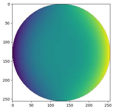
Note that we defined our grid to have a radius of 1, but often you may hold two copies of r, one which is normalized by some reference radius for polynomial evaluation, and one which is not for pupil geometry evaluation. The sign of the first argument can be made negative to generate a sine mode instead of cosine.
Zernike#
prysm has a fairly granular implementation of Zernike polynomials, and expects its users to assemble the pieces to synthesize higher order functionality. The basic building block is the zernike_nm function, which takes azimuthal and radial orders n and m, as in \(Z_n^m\). For example, to compute the equivalent “primary coma” Zernike mode as the hopkins example, one would:
[3]:
from prysm.polynomials import zernike_nm
cmaZ = zernike_nm(3, 1, r, t, norm=True)
cmaZ[mask]=np.nan
plt.imshow(cmaZ)
[3]:
<matplotlib.image.AxesImage at 0x7eb2b0b75f90>
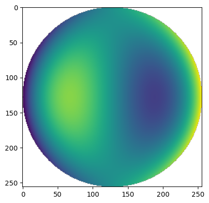
Note that the terms can be orthonormalized (given unit RMS) or not, based on the norm kwarg. The order m can be negative to give access to the sine terms isntead of cosine. If you wish to work with a particular ordering scheme, prysm supports Fringe, Noll, and ANSI out of the box, all of which start counting at 1.
[4]:
from prysm.polynomials import noll_to_nm, fringe_to_nm, ansi_j_to_nm

n, m = fringe_to_nm(9)
sphZ = zernike_nm(n, m, r, t, norm=False)
sphZ[mask]=np.nan
plt.imshow(sphZ)
[4]:
<matplotlib.image.AxesImage at 0x7eb2b0bf87d0>
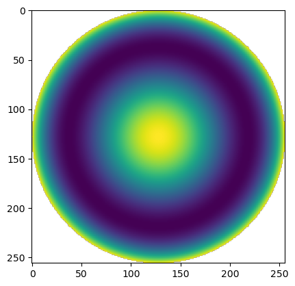
These functions are not iterator-aware and should be used with, say, a list comprehension.
If you wish to compute Zernikes much more quickly, the underlying implementation in prysm allows the work in computing lower order terms to be used to compute the higher order terms. The Zernike polynomials are fundamentally two “pieces” which get multiplied. The radial basis is where much of the work lives, and most programs that do not type out closed form solutions use Rodrigues’ technique to compute the radial basis:
prysm does not do this, and instead uses the fact that the radial polynomial is a Jacobi polynomial under a change-of-basis:
And the jacobi polynomials can be computed using a recurrence relation:
In other words, for a given \(m\), you can compute \(R\) for \(n=3\) from \(R\) for \(n=2\) and \(n=1\), and so on until you reach the highest value of N. Because the sum in the Rodrigues formulation is increasingly large as \(n,m\) grow, it has worse than linear time complexity. Because the recurrence in Eq. (3) does not change as \(n,m\) grow it does have linear time complexity.
The use of this recurrence relation is hidden from the user in the zernike_nm function, and the recurrence relation is for a so-called auxiliary polynomial (\(R\)), so the Zernike polynomials themselves are not useful for this recurrence. You can make use of it by calling the zernike_nm_seq function, a naming that will become familiar by the end of this reference guide. Consider the first 36 Fringe Zernikes:
[5]:
from prysm.polynomials import zernike_nm_seq

nms = [fringe_to_nm(i) for i in range(1,36)]

# zernike_nm_seq returns a cube of shape (len(nms), *r.shape)
%timeit basis = zernike_nm_seq(nms, r, t) # implicit norm=True
16.3 ms ± 121 μs per loop (mean ± std. dev. of 7 runs, 100 loops each)
Compare the timing to not using the seq flavored version:
[6]:
%%timeit
for n, m in nms:
    zernike_nm(n, m, r, t)
37.7 ms ± 333 μs per loop (mean ± std. dev. of 7 runs, 10 loops each)
There is no benefit other than performance to the _seq version of the function, but their usage is highly encouraged. A side benefit to the recurrence relation is that it is numerically stable to higher order than Rodrigues’ expression, so you can compute higher order Zernike polynomials without numerical errors. This is an especially useful property for using lower-precision data types like float32, since they will suffer from numerical imprecision earlier.
Orders, Sequences, and Derivatives#
Most families follow the same naming pattern:
foo(n, x)evaluates one order.foo_seq(ns, x)evaluates many orders, wherensshould be sorted in increasing order.foo_der(n, x)andfoo_der_seq(ns, x)evaluate analytic first derivatives.
The circular bases use (n, m) instead of only n, and the Cartesian XY basis uses (m, n) for the powers in x^m * y^n. Zernikes also have named index conversions for the common one-number orderings; XY has a one-number ordering for interoperability with optical design programs.
[7]:
from prysm.polynomials import (
    zernike_nm_der, zernike_nm_der_seq,
    zernike_nm_der_xy, zernike_nm_der_xy_seq,
    cheby1, cheby1_der, legendre_der,
    xy_j_to_mn,
)

print('Fringe 9 ->', fringe_to_nm(9))
print('Noll 6 ->', noll_to_nm(6))
print('ANSI 8 ->', ansi_j_to_nm(8))
print('XY j=8 ->', xy_j_to_mn(8))
Fringe 9 -> (4, 0)
Noll 6 -> (2, 2)
ANSI 8 -> (3, 1)
XY j=8 -> (2, 1)
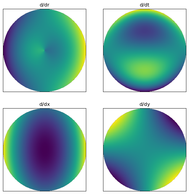
Derivatives are available in poly coordinates, as well as cartesian. Derivative sequence functions are also available
[8]:
dr, dt = zernike_nm_der(3, 1, r, t)

dx, dy = zernike_nm_der_xy(3, 1, x, y)

fig, axs = plt.subplots(ncols=2, nrows=2, figsize=(8,8))

labels = ['d/dr', 'd/dt', 'd/dx', 'd/dy']
ders = (dr, dt, dx, dy)
for ax, der, lab in zip(axs.ravel(), ders, labels):
    der[mask]=np.nan
    ax.imshow(der)
    ax.set(title=lab)
    ax.xaxis.set_visible(False)
    ax.yaxis.set_visible(False)
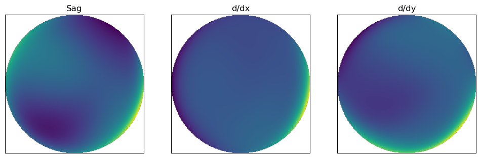
A bonus function is available which computes a weighted sum directly, as well as d/dx and d/dy. This is used in raytracing where the grid is not stable from call to call and the precomute basis then perform weighted sum approach used in the physical optics model cannot be used:
[9]:
from prysm.polynomials import zernike_sum_der_xy

# weighting to reduce amplitude of higher order modes
coef = np.random.rand(36) / (1+np.arange(36, dtype=float))**2
coef[:3]=0

# note takes x and y, not r, t
sag, dx, dy = zernike_sum_der_xy(coef, nms, x, y)
labels = ['Sag', 'd/dx', 'd/dy']
arrs = (sag, dx, dy)
fig, axs = plt.subplots(ncols=3, figsize=(12,4))

for ax, arr, lbl in zip(axs, arrs, labels):
    arr[mask]=np.nan
    ax.imshow(arr)
    ax.set(title=lbl)
    ax.xaxis.set_visible(False)
    ax.yaxis.set_visible(False)
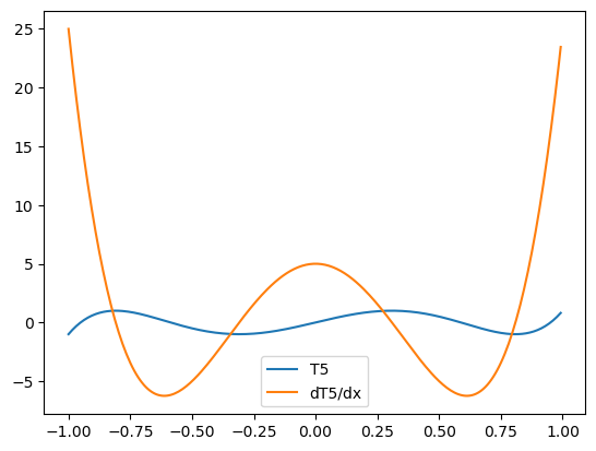
For one-dimensional bases, the derivative is with respect to x. For example, these two curves are a Chebyshev polynomial and its analytic derivative:
[10]:
x_ = x[0, :] # not required to be 1D, just for example
plt.plot(x_, cheby1(5, x_), label='T5')
plt.plot(x_, cheby1_der(5, x_), label='dT5/dx')
plt.legend()
[10]:
<matplotlib.legend.Legend at 0x7eb2b017af90>
Jacobi#
The Jacobi polynomials underly most other bases in the polynomial module.
[11]:
from prysm.polynomials import (
    jacobi,
    jacobi_seq,
    jacobi_der,
    jacobi_with_der,
    jacobi_seq_with_der,
    jacobi_der_seq,
    jacobi_sum_clenshaw,
    jacobi_sum_clenshaw_der
)
[12]:
x_ = x[0, :] # not required to be 1D, just for example
plt.plot(x_, jacobi_seq([1, 2, 3, 4, 5], 0, 0, x_).T)
[12]:
[<matplotlib.lines.Line2D at 0x7eb2b0259a90>,
 <matplotlib.lines.Line2D at 0x7eb2b0259be0>,
 <matplotlib.lines.Line2D at 0x7eb2b0259d30>,
 <matplotlib.lines.Line2D at 0x7eb2b0259e80>,
 <matplotlib.lines.Line2D at 0x7eb2b0259fd0>]
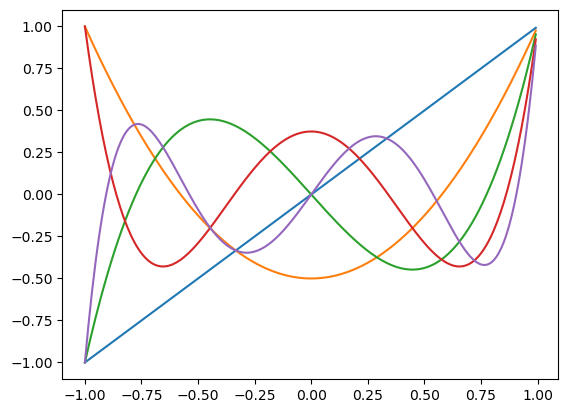
These shapes may be familiar to Zernike polynomials.
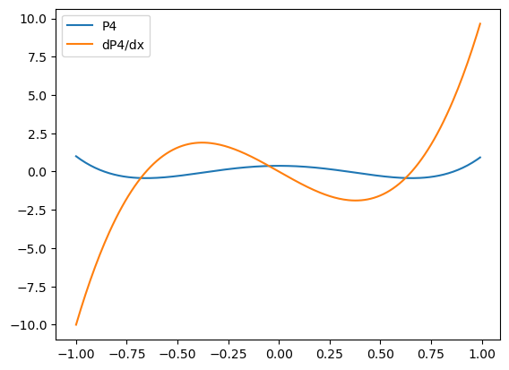
jacobi_with_der and jacobi_seq_with_der evaluate values and derivatives together when both are needed. This avoids computing the same recurrence twice. jacobi_sum_clenshaw and jacobi_sum_clenshaw_der compute the weighted sum or weighted sum and derivative in an accelerated single pass using a change of basis to Chebyshev polynomials and Clenshaw’s recursive method. This is the fastest possible technique to get the surface and its derivatives.
[13]:
vals, ders = jacobi_seq_with_der([1, 2, 3, 4, 5], 0, 0, x_)
plt.plot(x_, vals[3], label='P4')
plt.plot(x_, ders[3], label='dP4/dx')
plt.legend()
[13]:
<matplotlib.legend.Legend at 0x7eb2b00d7e00>
Chebyshev#
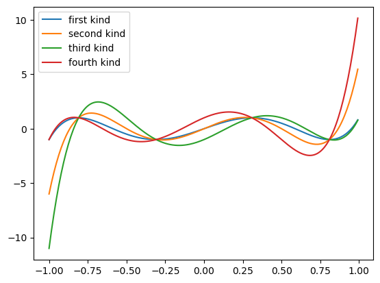
All four types of Chebyshev polynomials are supported. They are just special cases of Jacobi polynomials. The first and second kind are common:
While the third and fourth kind are more obscure:
[14]:
from prysm.polynomials import (
    cheby1, cheby1_seq, cheby1_der, cheby1_der_seq,
    cheby2, cheby2_seq, cheby2_der, cheby2_der_seq,
    cheby3, cheby3_seq, cheby3_der, cheby3_der_seq,
    cheby4, cheby4_seq, cheby4_der, cheby4_der_seq,
)
[15]:
fs = [cheby1, cheby2, cheby3, cheby4]
n = 5
for f in fs:
    plt.plot(x_, f(n,x_))
plt.legend(['first kind', 'second kind', 'third kind', 'fourth kind'])
[15]:
<matplotlib.legend.Legend at 0x7eb2a2f2a510>
Legendre#
These polynomials are just a special case of Jacobi polynomials:
Usage follows from the Chebyshev exactly, except the functions are prefixed by legendre. No plots here, they would be identical to Jacobi because the alpha and beta weights were zero in the jacobi example.
[16]:
from prysm.polynomials import legendre, legendre_seq, legendre_der, legendre_der_seq
Hermite#
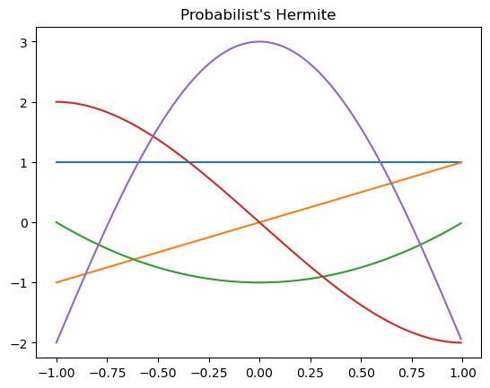
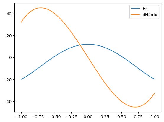
prysm includes both common Hermite conventions: probabilist’s \(He_n\) and physicist’s \(H_n\). Both have sequence and derivative variants.
[17]:
from prysm.polynomials import (
    hermite_He, hermite_He_seq, hermite_He_der, hermite_He_der_seq,
    hermite_H, hermite_H_seq, hermite_H_der, hermite_H_der_seq,
)

plt.plot(x_, hermite_He_seq([0, 1, 2, 3, 4], x_).T)
plt.title("Probabilist's Hermite")
[17]:
Text(0.5, 1.0, "Probabilist's Hermite")
[18]:
plt.plot(x_, hermite_H(4, x_), label='H4')
plt.plot(x_, hermite_H_der(4, x_), label='dH4/dx')
plt.legend()
[18]:
<matplotlib.legend.Legend at 0x7eb2a2e61be0>
Laguerre#
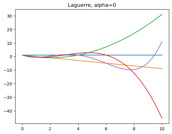
Generalized Laguerre polynomials use an order n and a shaping parameter alpha. They are orthogonal on \([0, \infty)\), so the example below uses a nonnegative coordinate vector.
[19]:
from prysm.polynomials import laguerre, laguerre_seq, laguerre_der, laguerre_der_seq

x_lag = np.linspace(0, 10, 256)
plt.plot(x_lag, laguerre_seq([0, 1, 2, 3, 4], alpha=0, x=x_lag).T)
plt.title('Laguerre, alpha=0')
[19]:
Text(0.5, 1.0, 'Laguerre, alpha=0')
Dickson#
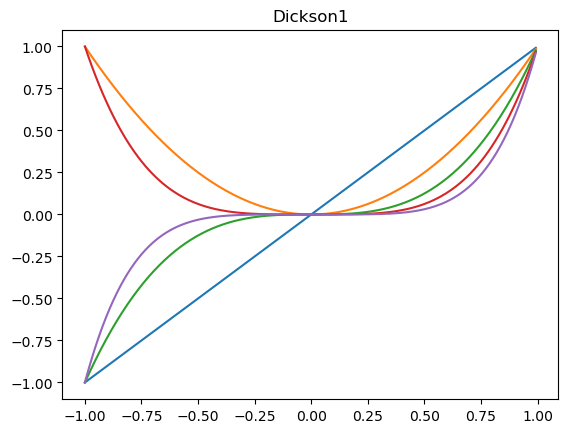
These polynomials use a two-term recurrence relation, but are not based on Jacobi polynomials. For the Dickson polynomials of the first kind \(D\):
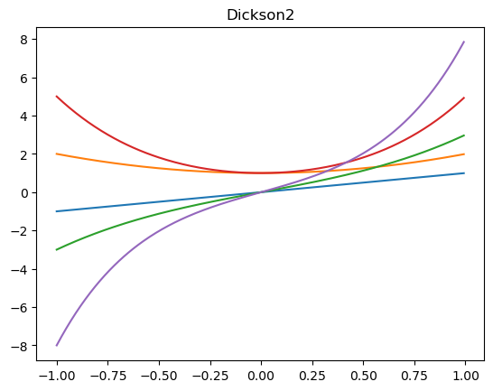
And the second kind \(E\):
The interface is once again the same:
[20]:
from prysm.polynomials import (
    dickson1, dickson1_seq, dickson1_der, dickson1_der_seq,
    dickson2, dickson2_seq, dickson2_der, dickson2_der_seq,
)
[21]:
x_ = x[0,:] # not required to be 1D, just for example
# dickson with alpha=0 are monomials x^n, or use alpha=-1 for Fibonacci polynomials
plt.plot(x_, dickson1_seq([1,2,3,4,5], 0, x_).T)
plt.title('Dickson1')
[21]:
Text(0.5, 1.0, 'Dickson1')
[22]:
x_ = x[0,:] # not required to be 1D, just for example
# dickson with alpha=0 are monomials x^n, or use alpha=-1 for Fibonacci polynomials
plt.plot(x_, dickson2_seq([1,2,3,4,5], -1, x_).T)
plt.title('Dickson2')
[22]:
Text(0.5, 1.0, 'Dickson2')
Qs#
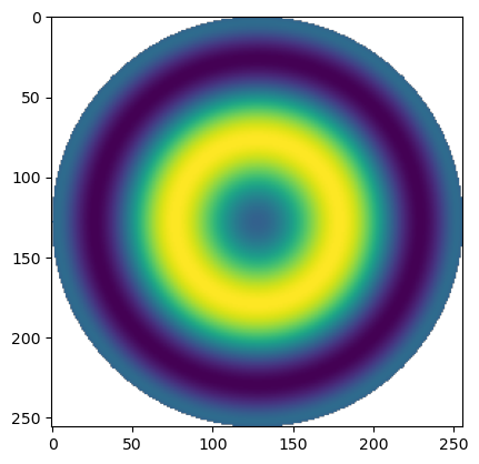
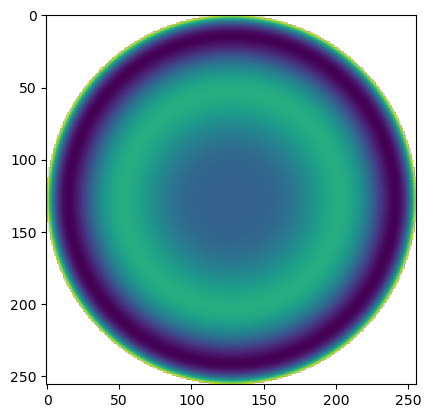
Qs are Greg Forbes’ Q polynomials, \(Q\text{bfs}\), \(Q\text{con}\), and \(Q_n^m\). Qbfs and Qcon polynomials are radial only, and replace the ‘standard’ asphere equation. The implementation of all three of these also uses a recurrence relation, although it is more complicated and outside the scope of this reference guide. Each includes the leading prefix from the papers:
\(\rho^2(1-\rho^2)\) for \(Q\text{bfs}\),
\(\rho^4\) for \(Q\text{con}\),
the same as \(Q\text{bfs}\) for \(Q_n^m\) when \(m=0\) or \(\rho^m \cos\left(m\theta\right)\) for \(m\neq 0\)
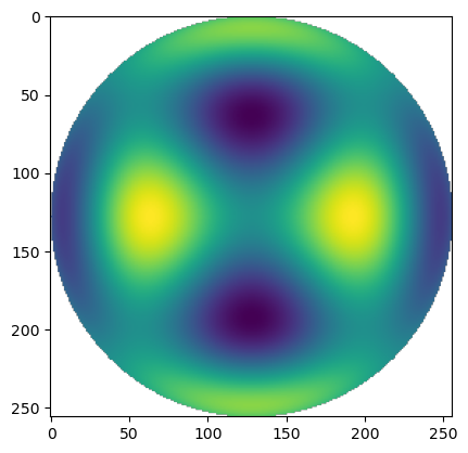
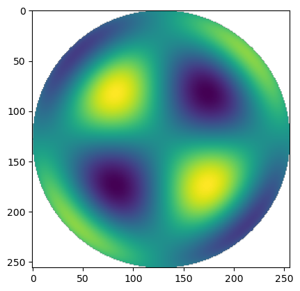
The \(Q_n^m\) implementation departs from the papers in order to have a more Zernike-esque flavor. Instead of having \(a,b\) coefficients and \(a\) map to \(\cos\) and \(b\) to \(\sin\), this implementation uses the sign of \(m\), with \(\cos\) for \(m>0\) and \(\sin\) for \(m<0\).
There are six essential functions:
[23]:
from prysm.polynomials import (
    Qbfs, Qbfs_seq, Qbfs_der, Qbfs_der_seq,
    Qcon, Qcon_seq, Qcon_der, Qcon_der_seq,
    Q2d, Q2d_seq, Q2d_der, Q2d_der_seq,
    Q2d_der_xy, Q2d_der_xy_seq,
)
[24]:
p = Qbfs(2,r)
p[mask]=np.nan
plt.imshow(p)
[24]:
<matplotlib.image.AxesImage at 0x7eb2a2cbd950>
[25]:
p = Qcon(2,r)
p[mask]=np.nan
plt.imshow(p)
[25]:
<matplotlib.image.AxesImage at 0x7eb2a2b07390>
[26]:
p = Q2d(2, 2, r, t) # cosine term
p[mask]=np.nan
plt.imshow(p)
[26]:
<matplotlib.image.AxesImage at 0x7eb2a2ba8e10>
[27]:
p2 = Q2d(2, -2, r, t) # sine term
p2[mask]=np.nan
plt.imshow(p2)
[27]:
<matplotlib.image.AxesImage at 0x7eb2a2a0e850>
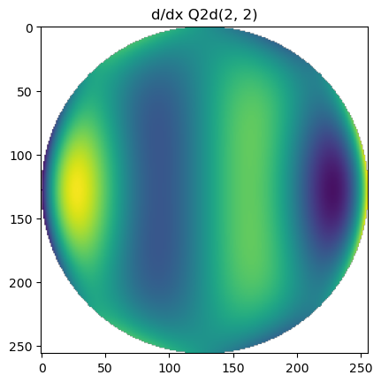
The Q derivative helpers follow the same split as Zernike: Q2d_der returns polar derivatives, while Q2d_der_xy returns Cartesian derivatives. The radial Qbfs and Qcon families have ordinary *_der helpers.
[28]:
qbfs_slope = Qbfs_der(2, r)
q_dr, q_dt = Q2d_der(2, 2, r, t)
q_dx, q_dy = Q2d_der_xy(2, 2, x, y)

q_dx = q_dx.copy()
q_dx[mask] = np.nan
plt.imshow(q_dx)
plt.title('d/dx Q2d(2, 2)')
[28]:
Text(0.5, 1.0, 'd/dx Q2d(2, 2)')
XY#
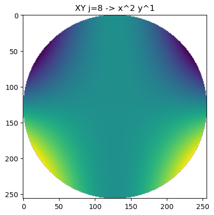
XY polynomials are implemented in the same manner as Code V. A monoindexing scheme that is identical to Code V (beginning from j=2) is provided. An additional j=1 term for piston (x^0 * y^0) is provided for easier use with the orthogonalization functions described later in this document:
[29]:
from prysm.polynomials import (
    xy, xy_seq, xy_j_to_mn,
    xy_der_x, xy_der_x_seq,
    xy_der_y, xy_der_y_seq,
    xy_der_xy, xy_der_xy_seq,
)

mns = [xy_j_to_mn(j) for j in range(1, 10)]
basis_xy = xy_seq(mns, x, y)

target_mn = xy_j_to_mn(8)
mode = basis_xy[mns.index(target_mn)].copy()
mode[mask] = np.nan
plt.imshow(mode)
plt.title(f'XY j=8 -> x^{target_mn[0]} y^{target_mn[1]}')
[29]:
Text(0.5, 1.0, 'XY j=8 -> x^2 y^1')
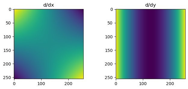
XY derivatives are named for the Cartesian partial derivative they compute: xy_der_x, xy_der_y, and the mixed partial xy_der_xy. Each also has a _seq version.
[30]:
m, n = xy_j_to_mn(8)
dx_xy = xy_der_x(m, n, x, y)
dy_xy = xy_der_y(m, n, x, y)

fig, axs = plt.subplots(ncols=2, figsize=(8, 3))
axs[0].imshow(dx_xy)
axs[0].set_title('d/dx')
axs[1].imshow(dy_xy)
axs[1].set_title('d/dy')
[30]:
Text(0.5, 1.0, 'd/dy')
Fitting#
lstsq performs a least-squares fit of a stack of modes to data. The data array is 2D, the modes are a sequence or array with shape (number_of_modes, *data.shape), and samples with NaN in the data are ignored. The least-squares fit works with all mode types, not only Zernikes.
[31]:
from prysm.polynomials import lstsq, sum_of_2d_modes

fit_nms = [noll_to_nm(j) for j in range(1, 12)]
fit_basis = zernike_nm_seq(fit_nms, r, t, norm=True)

true_coefs = np.zeros(len(fit_nms))
true_coefs[[3, 6, 8]] = [0.3, -0.08, 0.05]

data = sum_of_2d_modes(fit_basis, true_coefs)
data[mask] = np.nan

fit_coefs = lstsq(fit_basis, data)
print('true', true_coefs)
print('fit', fit_coefs)
print('err', true_coefs-fit_coefs)
true [ 0.    0.    0.    0.3   0.    0.   -0.08  0.    0.05  0.    0.  ]
fit [ 1.72253468e-16 -5.55111512e-17  6.76542156e-17  3.00000000e-01
  1.39794354e-17 -2.67820878e-17 -8.00000000e-02  4.33680869e-18
  5.00000000e-02 -3.72965547e-17 -2.77555756e-16]
err [-1.72253468e-16  5.55111512e-17 -6.76542156e-17 -3.33066907e-16
 -1.39794354e-17  2.67820878e-17  1.38777878e-17 -4.33680869e-18
  4.85722573e-17  3.72965547e-17  2.77555756e-16]
Error is at the floating point precision floor.
For an annulus or any arbitrary aperture, keep the same mode stack shape and mark samples outside the domain with NaN in data. lstsq applies the finite-data mask before solving the linear system.
Annular Domains#
prysm does not have explicit implementations of annular polynomials, for example Mahajan’s annular Zernikes. Because all of the polynomial routines recursively generate the basis sets based on the input coordinates, modifications of the grid will produce versions of the polynomials that are orthogonal over the new domain, such as an annulus. This underlying technique is actually how the radial basis of the Zernike polynomials is calculated. The coordinates module features a
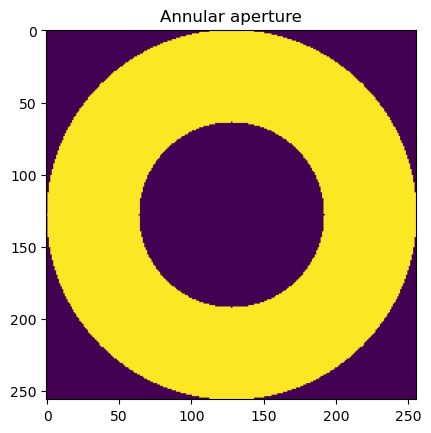
distort_annular_grid function that performs this modification to a circle. We will use it to show Annular Zernikes. We begin by making a circular aperture with huge central obscuration:
[32]:
eps = 0.5
maskod = circle(1, r)
maskid = circle(eps, r)
mask = maskod ^ maskid
plt.imshow(mask)
plt.title('Annular aperture')
[32]:
Text(0.5, 1.0, 'Annular aperture')
Then we compute a distorted grid and call the polynomial routines as you would in any other case. Note that the norm keyword argument uses analytic norms, which are not correct on distorted grids. A helper function is provided by the polynomials module, normalize_modes to enforce normalizations on modes.
[33]:
from prysm.coordinates import distort_annular_grid
from prysm.polynomials import normalize_modes
[34]:
x, y = make_xy_grid(mask.shape, diameter=2)
r, t = cart_to_polar(x, y)

ran = distort_annular_grid(r, eps)

# nms = [noll_to_nm(j) for j in range(1,12)] # up to primary spherical
js = range(1,36)
nms = [fringe_to_nm(j) for j in js]

basis = zernike_nm_seq(nms, ran, t, norm=False)
basis = normalize_modes(basis, mask, to='std')
# basis_in_ap = basis[:,mask]
# print(basis_in_ap.shape)
# std_per_coef = basis_in_ap.std(axis=1)

# newaxis broadcasts (11,) -> (11,1,1) for numpy broadcast semantics
# basis = basis * (1/std_per_coef[:,np.newaxis,np.newaxis])
fig, axs = plt.subplots(ncols=4, figsize=(12,3))
for ax, i, name in zip(axs, (3,4,6,8), ('Power', 'Astigmatism', 'Coma', 'Spherical Aberration')):
    mode = basis[i].copy()
    mode[~mask]=np.nan
    ax.imshow(mode, cmap='RdBu')
    ax.set(title=name)
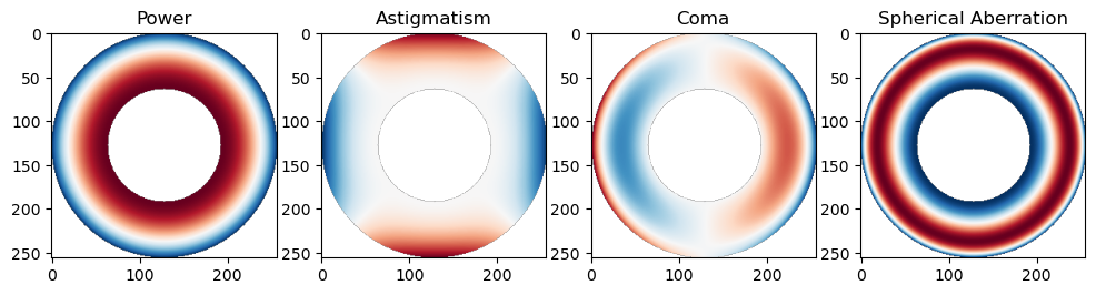
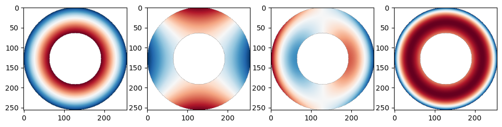
We can compare these distorted modes to ordinary Zernike polynomials:
[35]:
# note: r instead of ran, the undistorted grid
basis2 = zernike_nm_seq(nms, r, t, norm=False)
fig, axs = plt.subplots(ncols=4, figsize=(12,3))
for ax, i, name in zip(axs, (3,4,6,8), ('Power', 'Astigmatism', 'Coma', 'Spherical Aberration')):
    mode = basis2[i].copy()
    mode[~mask]=np.nan
    ax.imshow(mode, cmap='RdBu')
The same fitting pattern from the previous section applies here: use the annularly distorted and normalized basis, place NaN outside the annulus in the measured data, and call lstsq(basis, data).
Arbitrary Domains#
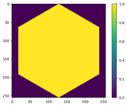
The grid distortion trick provided out-of-the-box for annular apertures is very easy to implement and use for an annulus, and similarly easy for an ellipse. More complex aperture shapes such as hexagons are less straightforward to derive a grid distortion for. For these use cases, or to provide an alternative orthogonalization approach for annular apertures, prysm features a QR factorization based orthogonalization approach over an arbitrary aperture. This is similar to performing a Gram-Schmidt process. We’ll repeat the annular example first:
[36]:
from prysm.polynomials import orthogonalize_modes
[37]:
basis3 = orthogonalize_modes(basis2, mask)
basis3 = normalize_modes(basis3, mask)

# purely cosmetic for plotting
nmask = ~mask
basis[:,nmask] = np.nan
basis2[:,nmask] = np.nan
basis3[:,nmask] = np.nan

fig, axs = plt.subplots(ncols=4, nrows=3, figsize=(12,9))
j = 0
for i, name in zip((3,4,6,8), ('Power', 'Astigmatism', 'Coma', 'Spherical Aberration')):
    raw_mode = basis2[i]
    grid_distorted_mode = basis[i]
    qr_mode = basis3[i]
    axs[0,j].imshow(raw_mode, cmap='RdBu')
    axs[1,j].imshow(grid_distorted_mode, cmap='RdBu')
    axs[2,j].imshow(qr_mode, cmap='RdBu')
    axs[0,j].set_title(name)
    j += 1

axs[0,0].set(ylabel='Circle Zernikes')
axs[1,0].set(ylabel='Annular Zernikes')
axs[2,0].set(ylabel='QR Orthogonalized Zernikes')

for ax in axs.ravel():
    ax.set_xticks([])
    ax.set_yticks([])
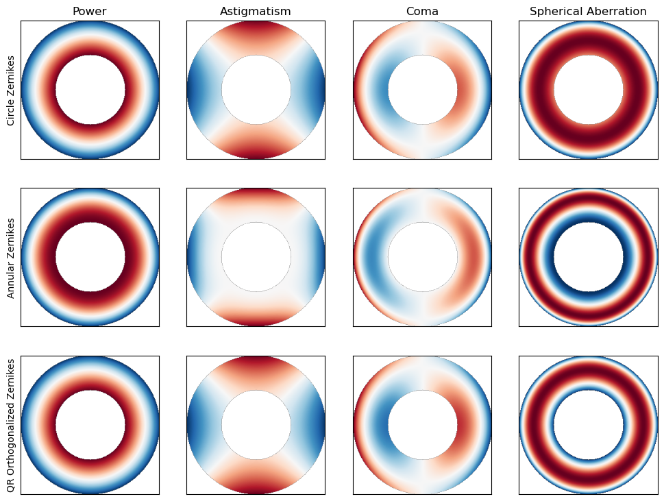
Note that both the basis generated by grid distortion and QR decomposition are orthogonal. In the same way that there are many orthogonal bases included in prysm, these are just different orthogonal sets derived from Zernike polynomials (which are themselves derived from Jacobi polynomials). We’ll now show a second example, for a hexagonal aperture:
[38]:
from prysm.geometry import regular_polygon
[39]:
hexap = regular_polygon(6, 1, x, y, rotation=0)
im = plt.imshow(hexap, interpolation='bilinear')
plt.colorbar(im)
[39]:
<matplotlib.colorbar.Colorbar at 0x7eb2a23af8c0>
[40]:
basis2 = zernike_nm_seq(nms, r, t, norm=True)
basis3 = orthogonalize_modes(basis2, hexap)
basis3 = normalize_modes(basis3, hexap, to='std')

# this masking is cosmetic only for plotting!
basis3[:, ~hexap] = np.nan

fig, axs = plt.subplots(ncols=4, nrows=2, figsize=(12,6))
j = 0
cl = (-3,3)
for i, name in zip((3,6,10,28), ('Power', 'Coma', 'Trefoil', 'Primary Quadrafoil')):
    raw_mode = basis2[i]
    raw_mode[~hexap] = np.nan
    qr_mode = basis3[i]
    axs[0,j].imshow(raw_mode, cmap='RdBu', clim=cl)
    axs[1,j].imshow(qr_mode, cmap='RdBu', clim=cl)
    axs[0,j].set_title(name)
    j += 1

axs[0,0].set(ylabel='Circle Zernikes')
axs[1,0].set(ylabel='QR Orthogonalized Zernikes')

for ax in axs.ravel():
    ax.set_xticks([])
    ax.set_yticks([])
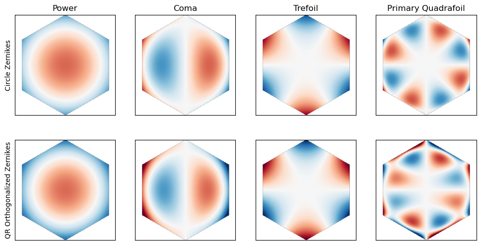
The similarity of the power, coma, and trefoil modes and dissimilarity of the higher order mode highlight a property of all polynomials: they are extremely similar, and largely irrespective of the domain for lower order modes. Higher order modes will distort significantly to match any given domain. If you are largely interested in lower order behaviors, orthogonality will likely not matter to you. It is only when concerned with higher order modes that orthogonality will be of significance.
An additional property of using QR factorization, Gram-Schmidt, SVD, or other processes to produce orthogonal bases is that the output mode shapes depends on every detail of the inputs. If the input basis changes, for example expanding Z1-Z11 in one case and Z1-Z36 in another, the output changes. Similarly, the normalization radius of the input Zernikes (if those are used) must be specified consistently, as well as the exact centering between the polynomials and the aperture. When the grid distortion techniques shown previously for annular apertures are used, the only relevant one of these effects is grid centering, which only impacts orthogonality and not mode shapes.
[ ]: