Ins and Outs of Polynomials
This document serves as a reference for how prysm is set up to work with polynomials, in the context of OPD or surface figure error. Much of what differentiates prysm’s API in this area has to do with the fact that it expects the grid to exist at the user level, but there are some deep and consequential implementation differences, too. Before we get into those, we will create a working grid and a mask for visualization:
[1]:
import numpy as np

from prysm.coordinates import make_xy_grid, cart_to_polar
from prysm.geometry import circle

from matplotlib import pyplot as plt

x, y = make_xy_grid(256, diameter=2)
r, t = cart_to_polar(x, y)
mask = circle(1,r) == 0
Matplotlib is building the font cache; this may take a moment.
This is a long document, so you may wish to search for your preferred polynomial flavor:
Note that all polynomial types allow evaluation for arbitrary order. First partial derivatives can be computed using the format {polynomial}_der or {polynomial}_der_sequence. 1D polynomials are differentiated with respect to x. 2D polynomials do not yet support differentiation. Differentiation is done analytically and does not rely on finite differences.
Hopkins
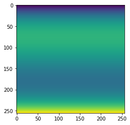
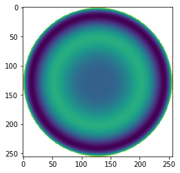
The simplest polynomials are Hopkins’:
for some set of coefficients. The usage of this should not be surprising, for \(W_{131}\), coma one can write:
[2]:
from prysm.polynomials import hopkins
cma = hopkins(1, 3, 1, r, t, 1)
cma[mask]=np.nan
plt.imshow(cma)
[2]:
<matplotlib.image.AxesImage at 0x7f3f003f4940>
Note that we defined our grid to have a radius of 1, but often you may hold two copies of r, one which is normalized by some reference radius for polynomial evaluation, and one which is not for pupil geometry evaluation. There is no further complexity in using Hopkins’ polynomials.
Zernike
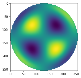
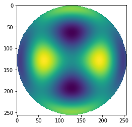
prysm has a fairly granular implementation of Zernike polynomials, and expects its users to assemble the pieces to synthesize higher order functionality. The basic building block is the zernike_nm function, which takes azimuthal and radial orders n and m, as in \(Z_n^m\). For example, to compute the equivalent “primary coma” Zernike mode as the hopkins example, one would:
[3]:
from prysm.polynomials import zernike_nm
cmaZ = zernike_nm(3,1, r,t, norm=True)
cmaZ[mask]=np.nan
plt.imshow(cmaZ)
[3]:
<matplotlib.image.AxesImage at 0x7f3f0036cb20>
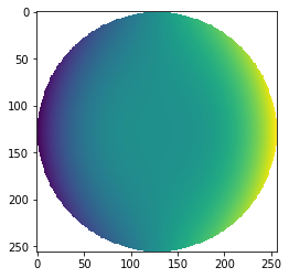
Note that the terms can be orthonormalized (given unit RMS) or not, based on the norm kwarg. The order m can be negative to give access to the sinusoidal terms instead of cosinusoidal. If you wish to work with a particular ordering scheme, prysm supports Fringe, Noll, and ANSI out of the box, all of which start counting at 1.
[4]:
from prysm.polynomials import noll_to_nm, fringe_to_nm, ansi_j_to_nm

n, m = fringe_to_nm(9)
sphZ = zernike_nm(n, m, r, t, norm=False)
sphZ[mask]=np.nan
plt.imshow(sphZ)
[4]:
<matplotlib.image.AxesImage at 0x7f3f002cd910>
These functions are not iterator-aware and should be used with, say, a list comprehension.
If you wish to compute Zernikes much more quickly, the underlying implementation in prysm allows the work in computing lower order terms to be used to compute the higher order terms. The Zernike polynomials are fundamentally two “pieces” which get multiplied. The radial basis is where much of the work lives, and most programs that do not type out closed form solutions use Rodrigues’ technique to compute the radial basis:
prysm does not do this, and instead uses the fact that the radial polynomial is a Jacobi polynomial under a change-of-basis:
And the jacobi polynomials can be computed using a recurrence relation:
In other words, for a given \(m\), you can compute \(R\) for \(n=3\) from \(R\) for \(n=2\) and \(n=1\), and so on until you reach the highest value of N. Because the sum in the Rodrigues formulation is increasingly large as \(n,m\) grow, it has worse than linear time complexity. Because the recurrrence in Eq. (3) does not change as \(n,m\) grow it does have linear time complexity.
The use of this recurrence relation is hidden from the user in the zernike_nm function, and the recurrence relation is for a so-called auxiliary polynomial (\(R\)), so the Zernike polynomials themselves are not useful for this recurrence. You can make use of it by calling the zernike_nm_sequence function, a naming that will become familiar by the end of this reference guide. Consider the first 16 Fringe Zernikes:
[5]:
from prysm.polynomials import zernike_nm_sequence

nms = [fringe_to_nm(i) for i in range(1,36)]

# zernike_nm_sequence returns a generator
%timeit polynomials = list(zernike_nm_sequence(nms, r, t)) # implicit norm=True
31.1 ms ± 86.2 µs per loop (mean ± std. dev. of 7 runs, 10 loops each)
Compare the timing to not using the sequence flavored version:
[6]:
%%timeit
for n, m in nms:
    zernike_nm(n, m, r, t)
101 ms ± 831 µs per loop (mean ± std. dev. of 7 runs, 10 loops each)
The sequence function returns a generator to leave the user in control of their memory usage. If you wished to compute 1,000 Zernike polynomials, this would avoid holding them all in memory at once while still improving performance. These is no benefit other than performance and plausibly reduced memory usage to the _sequence version of the function. A side benefit to the recurrence relation is that it is numerically stable to higher order than Rodrigues’ expression, so you can compute
higher order Zernike polynomials without numerical errors. This is an especially useful property for using lower-precision data types like float32, since they will suffer from numerical imprecision earlier.
Jacobi
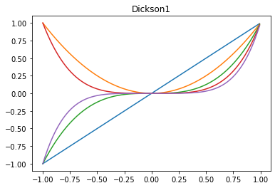
Of course, because the Zernike polynomials are related to them you also have access to the Jacobi polynomials:
[7]:
from prysm.polynomials import jacobi, jacobi_sequence

x_ = x[0,:] # not required to be 1D, just for example
plt.plot(x_, np.array(list(jacobi_sequence([1,2,3,4,5],0,0,x_))).T)
[7]:
[<matplotlib.lines.Line2D at 0x7f3f00248ca0>,
 <matplotlib.lines.Line2D at 0x7f3f00248c40>,
 <matplotlib.lines.Line2D at 0x7f3f00248d60>,
 <matplotlib.lines.Line2D at 0x7f3f00248e80>,
 <matplotlib.lines.Line2D at 0x7f3f00248fa0>]
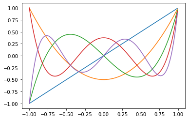
These shapes may be familiar to Zernike polynomials.
Chebyshev
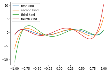
All four types of Chevyshev polynomials are supported. They are just special cases of Jacobi polynomials. The first and second kind are common:
While the third and fourth kind are more obscure:
[8]:
from prysm.polynomials import cheby1, cheby2, cheby1_sequence, cheby3, cheby4
[9]:
fs = [cheby1, cheby2, cheby3, cheby4]
n = 5
for f in fs:
    plt.plot(x_, f(n,x_))
plt.legend(['first kind', 'second kind', 'third kind', 'fourth kind'])
[9]:
<matplotlib.legend.Legend at 0x7f3f00208880>
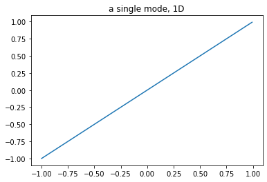
The most typical use of these polynomials in optics are as an orthogonal basis over some rectangular aperture. The calculation is separable in x and y, so it can be reduced from scaling by \(2(N\cdot M)\) to just \(N+M\). prysm will compute the mode for one column of x and one row of y, then broadcast to 2D to assemble the ‘image’. This introduces three new functions:
[10]:
from prysm.polynomials import separable_2d_sequence, mode_1d_to_2d, sum_of_xy_modes
[11]:
# orders 1, 2, 3 in x and 4, 5, 6 in y
ns = [1, 2, 3]
ms = [4, 5, 6]
modesx, modesy = separable_2d_sequence(ns, ms, x, y, cheby1_sequence)
plt.plot(x_, modesx[0]) # modes are 1D
plt.title('a single mode, 1D')
plt.figure()
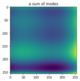
# and can be expanded to 2D
plt.imshow(mode_1d_to_2d(modesx[0], x, y))
plt.title('a single mode, 2D')
Wx = [1]*len(modesx)
Wy = [1]*len(modesy)
im = sum_of_xy_modes(modesx, modesy, x, y, Wx, Wy)
plt.imshow(im)
plt.title('a sum of modes')
[11]:
Text(0.5, 1.0, 'a sum of modes')
As a final note, there is no reason you can’t just use the cheby1/cheby2 functions with 2D arrays, it is only slower:
[12]:
im = cheby2(3, y)
plt.imshow(im)
[12]:
<matplotlib.image.AxesImage at 0x7f3f000472b0>
Legendre
These polynomials are just a special case of Jacobi polynomials:
Usage follows from the Chebyshev exactly, except the functions are prefixed by legendre. No plots here - they would be identical to those from the Jacobi section.
[13]:
from prysm.polynomials import legendre, legendre_sequence
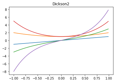
Dickson
These polynomials use a two-term recurrence relation, but are not based on Jacobi polynomials. For the Dickson polynomials of the first kind \(D\):
And the second kind \(E\):
The interface is once again the same:
[14]:
from prysm.polynomials import (
    dickson1, dickson1_sequence,
    dickson2, dickson2_sequence
)
[15]:
x_ = x[0,:] # not required to be 1D, just for example
# dickson with alpha=0 are monomials x^n, or use alpha=-1 for Fibonacci polynomials
plt.plot(x_, np.array(list(dickson1_sequence([1,2,3,4,5], 0, x_))).T)
plt.title('Dickson1')
[15]:
Text(0.5, 1.0, 'Dickson1')
[16]:
x_ = x[0,:] # not required to be 1D, just for example
# dickson with alpha=0 are monomials x^n, or use alpha=-1 for Fibonacci polynomials
plt.plot(x_, np.array(list(dickson2_sequence([1,2,3,4,5], -1, x_))).T)
plt.title('Dickson2')
[16]:
Text(0.5, 1.0, 'Dickson2')
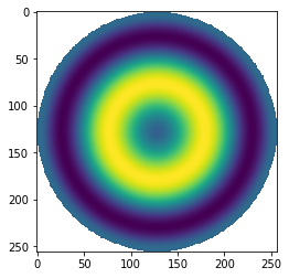
Qs
Qs are Greg Forbes’ Q polynomials, \(Q\text{bfs}\), \(Q\text{con}\), and \(Q_n^m\). Qbfs and Qcon polynomials are radial only, and replace the ‘standard’ asphere equation. The implementation of all three of these also uses a recurrence relation, although it is more complicated and outside the scope of this reference guide. Each includes the leading prefix from the papers:
\(\rho^2(1-\rho^2)\) for \(Q\text{bfs}\),
\(\rho^4\) for \(Q\text{con}\),
the same as \(Q\text{bfs}\) for \(Q_n^m\) when \(m=0\) or \(\rho^m \cos\left(m\theta\right)\) for \(m\neq 0\)
The \(Q_n^m\) implementation departs from the papers in order to have a more Zernike-esque flavor. Instead of having \(a,b\) coefficients and \(a\) map to \(\cos\) and \(b\) to \(\sin\), this implementation uses the sign of \(m\), with \(\cos\) for \(m>0\) and \(\sin\) for \(m<0\).
There are six essential functions:
[17]:
from prysm.polynomials import (
    Qbfs, Qbfs_sequence,
    Qcon, Qcon_sequence,
    Q2d, Q2d_sequence,
)
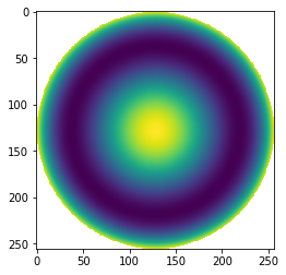
[18]:
p = Qbfs(2,r)
p[mask]=np.nan
plt.imshow(p)
[18]:
<matplotlib.image.AxesImage at 0x7f3ef9f7a040>
[19]:
p = Qcon(2,r)
p[mask]=np.nan
plt.imshow(p)
[19]:
<matplotlib.image.AxesImage at 0x7f3ef9edd130>
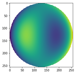
[20]:
p = Q2d(2, 2, r, t) # cosine term
p[mask]=np.nan
plt.imshow(p)
[20]:
<matplotlib.image.AxesImage at 0x7f3ef9eb6280>
[21]:
p2 = Q2d(2, -2, r, t) # sine term
p2[mask]=np.nan
plt.imshow(p2)
[21]:
<matplotlib.image.AxesImage at 0x7f3ef9e24310>