How prysm Works

This notebook will walk through how prysm works, so that users can develop intuition for the library.

Imports

prysm is structured into many sub-modules; common practice is to import that needed pieces and not use star imports. See the bottom of the next section for an example.

Grids

All functions in prysm operate on arrays, taking the relevant coordinates as arguments, e.g. \(x\) and \(y\) or \(\rho\) and \(\theta\). No functions take anything like sample_count or npix as arguments. This is to keep the library simple, and prevent any disagreement on assumptions about whether an array is inter-sample centered (not containing a zero element for even-size arrays) or fft-centered (containing a zero element always). It is not meaningfully different to pass npix everywhere or pass x, y.

For example, if you want to evaluate polynomials on a grid you already have handy, you would just import the relevant function(s). Here make_xy_grid and cart_to_polar are imported to create the grid, but they operate on and return ordinary arrays and are not special.

from prysm.coordinates import make_xy_grid, cart_to_polar
from prysm.polynomials import zernike_nm

from matplotlib import pyplot as plt

x, y = make_xy_grid(256, diameter=2)
r, t = cart_to_polar(x, y)

focus = zernike_nm(4, 0, r, t)
plt.imshow(focus)

<matplotlib.image.AxesImage at 0x7fd7dc44c070>

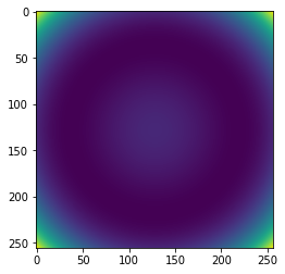
We will gloss over for a moment that the Zernike polynomials are orthogonal over the unit disk and the image contains points outside that domain.

Many problems have multiple planes which require different grids. For example, a simple image chain problem has three principle grids; that for the pupil, for the PSF, and for the Fourier domain of the PSF. These must all be managed separately. The `image chain modeling <>`__ tutorial shows an example of this.

Functions and Types

If you use prysm for physical optics, you will find that it is predominantly composed of functions which the user can combine into higher level concepts with relatively few classes. This is a conscious choice; we believe that it is easier to learn functions than type systems, and functions are often more composable than types, allowing fine-grained control of what operations are performed.

If you have used some other physical optics programs before, you may be familiar with their concept of a Wavefront (PROPER) which is modified as you navigate the system, and all functions operate on the wavefront. Similarly, POPPY has a concept of an OpticalSystem which sets up the problem. These types are black boxes and difficult to penetrate. Equivalent functionality is achieved in prysm by the user passing grids and other data around as function arguments. For example, if you want to set up a model of a system with a circular aperture and some polynomial-based wavefront error, you would use functions from prysm or your own. to build the grids, functions to build the transmission function, and functions to build the phase error.

To do any of these things, you need know nothing about any of the others, and there is no compromise or complexity introduced into any of them by the others.

In this way, any slow calculations that need not be in loops may easily be kept out of loops by the user, an any repetitive calculations may be cached by the user without introducing any complexity into the underlying software.

dx, or x?

Some types in prysm have constructors which take args of x, y while others take dx. prysm assumes rectilinear sampling, and dy == dx is implicitly assumed. Essentially, optical propagation does not require knowledge of all of the coordinates so prysm does not track it. However, some other calculations (like masking interferograms) does require full knowledge of the grid, so these types track x and y.